How to weight survey data with a dyadic multi-actor design?

Special issue

---

Abstract

This paper deals with adjustment for nonresponse in dyadic multi-actor survey designs. It presents a multi-dimensional approach to weighting that addresses the various analytical units represented in such data, so that sampling design weights are correctly accounted for and so that consistency between weights is achieved. This approach is demonstrated by using the primary respondents in the Divorce in Flanders study, which is a typical example of a dyadic multi-actor design. Five sets of weighting coefficients are made available whereby different subsets of data, according to different analytical units, are selected: the subset of the dyads, the subset of men and women respectively, and two subsets of marriages. Post-stratification – with the year of marriage, status of the reference marriage at the sampling date and five-year divorce cohort as auxiliary variables – was chosen as the weighting adjustment technique.

Keywords

dyadic data, dyadic sampling unit, multi-actor survey, nonresponse bias, weighting adjustment techniques

Acknowledgement

This study has been funded by the Flemish Agency for Innovation by Science and Technology (IWT grant agreements no.060071 and no. 080039 for the Divorce in Flanders project)

Introduction

This paper describes how post-stratification can be applied to a dyadic multi-actor survey design. Surveys with this design use dyads as primary respondents, directly sampled from the sampling frame, and possibly surrounded by secondary respondents for whom contact information is made available by the primary respondents (Pasteels & Mortelmans, 2013). Analogous to surveys of individuals, those using a multi-actor design also suffer from unit nonresponse, meaning that not all the selected individuals participate in the study with the result that the net sample deviates from the gross sample. For a description of general correlates of nonresponse, we refer to Groves and Couper (1998), Groves et al. (2002), Stoop (2005) and Stoop et al. (2010). Whether this deviation is harmful, depends on the type of missing data. Distinguishing between data missing completely at random (MCAR), data missing at random (MAR) and data not missing at random (NMAR) disentangles the phenomenon of unit nonresponse and shows how missing data can cause bias in the estimators (which it probably will), but fortunately, it also proves that bias can be corrected in some cases (Bethlehem et al., 2011).

However, this well-known typology of missing data, which classifies nonresponse with regard to the problem of selectivity, does not cover all the dimensions of the unit nonresponse problem in multi-actor survey designs. Before exploring selective nonresponse in a multi-actor survey, it is necessary to be aware that the problem of missing data is also characterized by the extent of unit nonresponse that can vary across multi-actor units. Moreover, weighting multi-actor designs is more difficult than standard designs for four reasons. First, sampling designs are more complex and so are design weights. Second, consistency in weights between the various units and levels has to be obtained. Third, relevant auxiliary information may come in different forms for the various units and levels. Last, there is an inherent longitudinal nature to these designs, which complicates any adjustment.

In this paper, we shed light on the use of post-stratification as a suitable weighting adjustment technique, given the complex sample design, and we deal with the issue of consistency between weighting coefficients for different analytical units. Therefore, we explain how a dyadic multi-actor design leads to a wider range of analytical units compared with surveys of individuals or households. This means that nonresponse has to be considered on the different levels, and multi-dimensional weighting procedures have to be carried out in order to make the data representative for all the different analytical levels. Our aim here is to develop a conceptual framework in order to deal with the nonresponse problem given the specificities of a multi-actor design. By demonstrating and conceptualizing how post-stratification can be applied in a dyadic multi-actor survey, in view of the different analytical strategies and the corresponding entries in a multi-actor database, we will add something new to existing literature.

For this purpose, we introduce some new terminology with regard to multi-actor survey designs. Next, we shed light on the different analytical levels that characterize multi-actor data and we present appropriate response rates. After a short overview of post-stratification as a weighting adjustment technique, we provide a set of formulas in order to calculate weighting coefficients that deal with selective nonresponse in three different ways. Finally, we show how these calculations have to be carried out on all the analytical levels that can be distinguished, given a dyadic multi-actor design. As it is an example of a survey with a multi-actor design, we use data from the Divorce in Flanders (DIF) study (Mortelmans et al., 2012). We start by presenting the DIF study so that all the theoretical considerations can immediately be illustrated using this survey.

 

Data

The fieldwork for the Divorce in Flanders study was carried out between September 2009 and December 2010. As the title suggests, DIF is a survey on the consequences of divorce in Flanders, the Northern region of Belgium. The main target of this study was questioning both parties in the divorce. This was not a mere gender-related choice designed to provide a ‘his and her’ look at divorce. Instead, the basic aim was to have insights into both partners’ viewpoints on the divorce process and to compare the subsequent consequences. For this purpose, the most appropriate design was a multi-actor study, in which both ex-partners were included. Divorcees were the main focus of interest and couples who were still married were sampled as a control group. In this paper, we refer to spouses and ex-spouses as ‘partners’, although they may be divorced.

Couples and former couples who married between 1971 and 2008 were sampled. Each partner was contacted by an interviewer, regardless of the participation of the other. In addition, one parent of each partner, a common own resident or non-resident child and new partners in the case of divorce, were invited to participate. The sampling frame for selecting both partners was the Belgian National Register. The target population of this study consisted of people in a legally recognized marriage that fulfilled 10 criteria (for more details see Pasteels et al., 2012). Two of the criteria for the sampling design are of major importance regarding the weighting procedure. First, the marriage was entered into between 1 January 1971 and 31 December 2008 and second, it was a marriage between different-sex partners.

Two key ideas were important to shape the design of the gross sample. On the one hand, a proportional distribution by the year of marriage was considered. On the other hand, it was preferable that divorced couples were over-represented in the sample, given the nature of the information the survey aimed to provide. Therefore, the year of marriage and the marital status at the time the sample was drawn were used as relevant stratification criteria. The sample was drawn proportionally to the year of the marriage within each subgroup of intact and dissolved reference marriages respectively. This means that the proportion of reference marriages from a specific year in the gross sample for each subgroup was the same as in the general population.

The objective of the survey was to obtain 2,000 completed double interviews of divorced couples and 1,000 completed double interviews of still-married couples. The term ‘double interview’ was introduced during the fieldwork in order to indicate the linked information for two partners from the same reference marriage. In cases when only one partner from a reference marriage was included, the term ‘single interview’ is used. Based on known response figures for Belgian and Flemish individual and household surveys (the Generations and Gender Survey [GGS]; the Survey of Health, Ageing and Retirement in Europe [SHARE]; the Health Interview Survey [HIS]), a gross sample of about 2,500 intact and 6,000 non-intact reference marriages was requested from the National Register.

Terminology

To deal with the multi-actor design, we use a conceptual framework presented in previous work (Pasteels & Mortelmans, 2013). In surveys with this design, several individuals are involved who are related to each other by precisely-defined social ties. All individuals, together with the defined social relationships and social roles, characterize and constitute a multi-actor scheme. In other words, the multi-actor unit joins all individuals in their different roles. By using this definition, we opt to broaden the more often applied notion of multi-actor surveys as being surveys with several members of the same family, who do not necessarily live in the same household (Stoop, 2012). We define multi-actor surveys in a more abstract way, as settings other than a family can also be examined using a multi-actor design, for example an educational system with pupils, teachers and parents as the main actors, or labour-force settings with employers and employees.

Furthermore, we have stated that a multi-actor design also defines the sampling unit. Because sampling frames for entire multi-actor units – with information about all individuals and the according social ties under consideration – are rarely available, the sampling unit differs from the multi-actor unit. The sample unit defines how the sample for a multi-actor survey will be drawn. If the sample unit comprises only one directly selected individual, around whom the remaining multi-actor pattern will be built, survey data is considered as being ‘singular multi-actor data’. If several people are directly sampled, survey data is ‘multiple multi-actor data’. In the case of two directly sampled individuals, we refer to the type of survey data as ‘dyadic multi-actor data’ (Pasteels & Mortelmans, 2013). We add to this terminology the idea of non-interchangeability as being characteristic of a multiple sampling unit, meaning that all people in a sampling unit are uniquely defined and accordingly are distinguishable from each other.

From a data collection perspective, primary and secondary respondents can be distinguished in a multi-actor design (Kalmijn & Liefbroer, 2011). Primary respondents are individuals directly sampled as members of a known population for which a sampling frame and associated contact information is available. Secondary respondents are those who are not directly selected from a sampling frame, but for whom information has to be provided by the primary respondents.

Figure 1 shows how this terminology can be applied to the Divorce in Flanders study. The multi-actor unit and the sampling unit are indicated. The multi-actor unit consists of all individuals who are connected with each other through the first marriage of both partners by the relationships and corresponding selection rules that are explicitly determined in the design. The two partners are the primary respondents. Parents, children and new partners are the secondary respondents. Therefore, the sampling unit consists of both partners in the first marriage. DIF can accordingly be considered as a dyadic multi-actor survey. Moreover, since only heterosexual marriages were selected, we clearly distinguish a male and a female partner within the sampling unit. This means that the primary respondents who comprise the sampling unit in the DIF study, are non-interchangeable.

 

Figure 1. Divorce in Flanders study: sampling unit and multi-actor unit

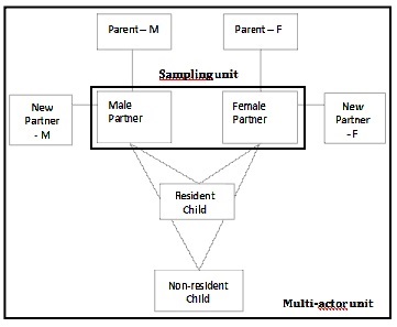
Source: Divorce in Flanders, 2010.

In this paper, we restrict the application of the weighting adjustment theory to a survey with a dyadic multi-actor design, having as the sampling unit, two primary respondents who are related to each other by pre-defined social ties. Moreover, we exclusively focus on the partners as the primary respondents. Applying post-stratification for secondary respondents (children, parents and new partners) is beyond the scope of this paper.

 

Different analytical levels and response rates in dyadic multi-actor surveys

Given a dyadic multi-actor design with two directly selected primary respondents, four analytical levels can be differentiated. First, treating the dyad as an analytical unit is self-evident, given the design. Second, the primary respondents, if distinguishable from each other, can also be considered as two separate analytical units. Last, analogous to surveys of individuals, all the primary respondents together can be seen as selected respondents from the same population and consequently, they can be considered as individuals representing the sample unit. In other words, the individual is representative of the marriage. Of course, the clustering of these individual units within the dyad is one of the key challenges when analysing data from surveys with a dyadic multi-actor design.

These four analytical units correspond to four different subsets that can easily be retrieved from the entire database, but in each different subset, the population distribution on substantively relevant variables has to be reproduced in order to obtain unbiased estimators for outcome variables. Consequently, in the case of selective nonresponse, all subsets require appropriate weighting coefficients, meaning that a multi-dimensional weighting adjustment procedure has to be carried out.

For the DIF study, the four analytical levels within the multi-actor design are: (1) couples or dyads of male and female partners, (2) male partners, (3) female partners and (4) marriages, whereby each marriage is represented by at least one individual, being either the male partner, the female partner or both. Figure 2 shows which subsets, according to these four levels of analysis, can be retrieved from the multi-actor database.

 

 

Figure 2.  Four analytical levels and corresponding subsets of the dyadic multi-actor survey Divorce in Flanders

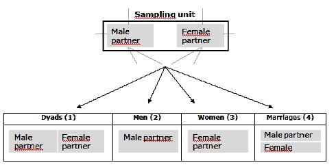
Source: Divorce in Flanders, 2010

 

Response rates can be calculated for each different analytical level. Table 1 shows the response rates for the final Divorce in Flanders dataset. Analogous to surveys on individuals, the response rate at the individual level indicates how many of all the selected individual partners participated in the study, by adding together the numbers of male and female respondents. In addition to response rates at the individual level, response rates referring to a different extent of attrition within the dyad can also be considered. These outcomes show the extent to which the multi-actor design can be realized. We use four response indicators corresponding with the four analytical levels mentioned before: the percentage of complete data for the dyad, meaning that both partners participated in the study (1), the response percentages of men (2) and women (3) respectively – each being one uniquely defined part of the sampling unit – and the percentage of reference marriages that are represented by at least one individual in the dataset (4).

Table 1. Response rates of partners by status of the reference marriage, the individual level and the multi-actor level

	Intact		Non-intact		Total
	N	%	N	%	N	%
INDIVIDUAL LEVEL
Selected partners (gross sample)	5,004		12,004		17,008
Interviewed partners (net sample)	1,775	35%	4,590	38%	6,365	37%
MULTI-ACTOR LEVEL
Selected reference marriages (gross sample)	2,502		6,002		8,504
Dyads (interview of both partners)	769	31%	1,097	18%	1,866	22%	(1)
Men	818	33%	2,147	36%	2,965	35%	(2)
Women	957	38%	2,443	41%	3,400	40%	(3)
Marriages (interview of at least one partner)	1,006	40%	3,493	58%	4,499	53%	(4)

 

Source: Divorce in Flanders, 2010.

At the individual level, 37 per cent of all selected people participated in the survey. For 22 per cent of all selected marriages a double interview was realized. Some 35 per cent of men and 40 per cent of women participated in the study. The 6,365 completed interviews represent 53 per cent of all selected marriages. The differences between intact and non-intact marriages are notable. For dissolved marriages, 58 per cent are represented in the dataset, whereas for intact marriages the number where at least one partner participated is only 40 per cent. By contrast, dyadic data for only 18 per cent of non-intact marriages could be gathered, whereas dyads were obtained for 31 per cent of all intact marriages. Accordingly, although the sample size was chosen with the objective of obtaining 2,000 dyads from the gross sample of divorced couples and 1,000 dyads from married couples, we did not reach this intended goal. Both partners were interviewed for only 769 intact and 1,079 non-intact reference marriages. Last, and analogous to what has been found in most surveys, Table 1 shows that men are less likely to participate than women, regardless of whether or not they are divorced.

 

Selective nonresponse

As shown in Table 1, the response rates are low, so selective nonresponse has to be explored in depth. Given the multi-actor design, analysis of nonresponse has to be carried out for all analytical levels. Using the year of marriage as the first auxiliary variable, Figure 3 shows how well the different subsets of data from both subsamples – the intact (left) and non-intact reference marriages (right) – reproduce the distribution of the population. Each line in the graph represents one of the four subsets mentioned above. An extended description of the selective nonresponse is not given here, as it is more crucial to understand how to consider selective nonresponse in a multi-dimensional way, meaning that deviations between distributions of the population and all subunits have to be explored separately.

 

Figure 3. Distribution of population/gross sample and net samples by marriage year for intact (left) and non-intact reference marriages (right)

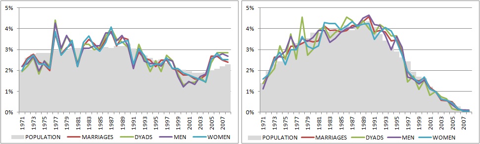
Source: Divorce in Flanders, 2010.

 

In addition to the year of marriage and status of the reference marriage at the time the sample was drawn (still married or ever divorced), the year of divorce categorized in intervals of five years was also used as an auxiliary variable. We chose this additional variable for substantive reasons. Many studies based on DIF data concern the subgroup of divorcees, for example studies about transitions in the post-marital life course or about the consequences of experiencing a divorce. The large time interval of marital cohorts under consideration (people entered their first marriage between 1971 and 2008), represents an extensive group of divorce cohorts. The divorce could have occurred at any time between 1971 and 2009. In order to explore selective nonresponse according to the time of divorce, we compared the realized distribution for five-year divorce cohorts with the original distribution in the population.

In Figure 4, each stratum according to a year of marriage is divided into substrata using the five-year divorce cohort information. In the graphs, the labels 1971 to 2008 refer to the year the marriage was entered into and the numbers 1 to 8 refer to eight divorce cohorts: 1971-1975, 1976-1980, 1981-1985, 1986-1990, 1991-1995, 1996-2000, 2001-2005 and 2006-2009. Again, the different curves show how the data for the four different subsets fits the distribution of the population when cross-tabulating year of marriage and five-year divorce cohort.

 

Figure 4. Distribution of population and net samples by marriage year and 5-year divorce cohort for non-intact marriages

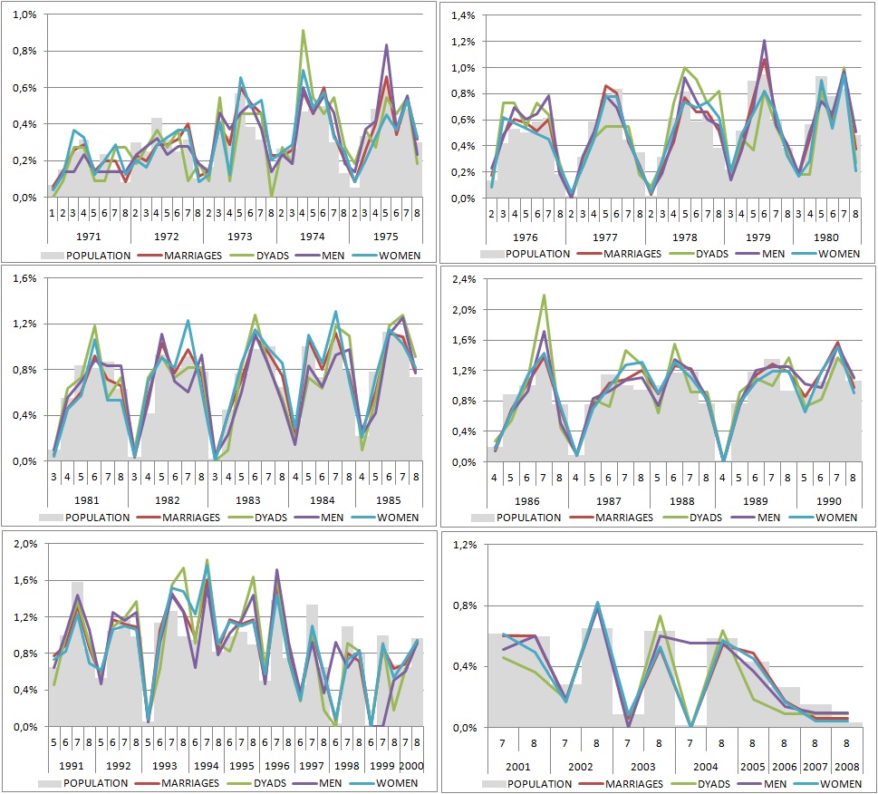
Legend 5-year divorce cohorts: 1=1971-1975, 2=1976-1980, 3=1981-1985, 4=1986-1990, 5=1991-1995, 6=1996-2000, 7=2001-2005, 8=2006-2009.

Source: Divorce in Flanders, 2010.

 

Weighting coefficients in the DiF – study

In this section, we show how post-stratification as a well-known weighting adjustment technique can be applied in surveys with a multi-actor design. Because the focus of this paper is not the question of which auxiliary variables would optimize the adjustment for nonresponse in divorce studies, we only present the weights in the DIF study that use information from the sampling frame – the Belgian National Register – as auxiliary information in the weighting procedure. The key ideas behind constructing these weighting coefficients can easily be applied using other auxiliary variables. All the information that is available for respondents and non-respondents can be considered as possible auxiliary variables (for more details about auxiliary variables see Särndal & Lundström [2005] and Schouten [2007]). As shown in Figure 3, Figure 4 and Figure 5, as auxiliary information we use both stratification variables (the marital status and the year of marriage) and additionally the year of divorce.

Two steps were necessary in order to calculate weighting coefficients for the Divorce in Flanders study. First, we had to take into account the complex sample design, characterized by the proportionality to year of marriage within each subgroup – each containing exclusively either intact or non-intact marriages – and simultaneously we had to consider the disproportionality to marital status across subgroups. Second, we had to deal with a dataset from which multiple analytical levels can be deduced, which is the main challenge for weighting multi-actor survey data.

 

Three different weighting coefficients

As a first step, we opted for post-stratification as a weighting adjustment technique in addition to design weights calculated as the inverse of the selection probability in the sample design (Kish, 1965; Lohr, 2010). Several weighting adjustment techniques are described in relevant literature, such as post-stratification, linear weighting, multiplicative weighting, propensity weighting and calibration (Bethlehem et al., 2011; Cobben, 2009; Gelman & Carlin, 2002; Groves, 2006; Laaksonen & Chambers, 2006; Little, Rosenbaum & Rubin, 1984; 1986; Schouten, 2006; Schouten et al., 2009; Stoop et al., 2010; Vaillant et al., 2013). Post-stratification is the simplest and most commonly used weighting technique to adjust for selective nonresponse (Bethlehem et al, 2011). As an extensive review of post-stratification would be beyond the scope of this article, we simply summarize the key idea that is most relevant for our own study presented here.

The key idea of adjusting selective nonresponse in order to obtain unbiased estimators is that the inclusion weight d_i of the Horvitz-Thompson estimator is replaced by (d_i x g_i), with g_i being the correction weight produced by this weighting adjustment technique. In the case of post-stratification, a correction factor g_i is required to equalize the relative distribution of the strata of the net sample with the corresponding distribution of strata in the population. This factor g_i can be denoted by Formula 1, with N_h/N being the relative size of stratum h in the population and n_h/n being the relative size for the same stratum in the net sample (Bethlehem, 2011).

 

(Formula 1)

With marital status, the year of marriage and the time of divorce in five-year cohorts as the auxiliary variables, weighting adjustment for the Divorce in Flanders data was carried out by combining design weighting and post-stratification in three different ways. Formulas 2 to 4 show the calculations.

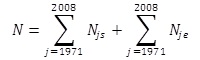
First, design weighting was applied for still married and ever-divorced couples respectively (see also Figure 3). Formula 2 shows how the weighting coefficients for both subsamples were calculated in order to reproduce the proportionality according to the year of marriage. Indices s and e refer to the subsamples of still married and ever divorced couples respectively, and index j corresponds to the year of marriage. N_s is the number of all reference marriages with still-married partners in the population and N_e is the number of all reference marriages in the population with partners who had ever divorced. N_js and N_je are the corresponding numbers of reference marriages for both subgroups within each marital year. Notations n_s, n_e, n_js and n_je refer to all the corresponding numbers in the net sample.

 

		and		(Formula 2)
	with          j = 1971, 1972, …, 2008

 

Second, as data providers for this project, we decided to post-stratify on divorce cohort so that representativeness of the data regarding the timing of the divorce is guaranteed for researchers carrying out future studies. To keep the number of strata limited and the observed cell sizes large enough, we post-stratified by using five-year intervals (see also Figure 4). The post-stratification according to divorce cohorts was carried out in addition to the reproduction of the proportionality according to year of marriage. Formula 3 shows how the weighting coefficients for both subsamples were calculated in order to reproduce the proportionality according to year of marriage and also in the case of divorce, according to five-year divorce cohorts. Index k refers to the five-year divorce cohorts, with the intervals 1971-1975, 1976-1980, 1981-1985, 1986-1990, 1991-1995, 1996-2000, 2001-2005 and 2006-2009.

 

			and		(Formula 3)
	with               j = 1971, 1972, …, 2008
		k= j, j+1,…. , 2009 recoded in 5-year divorce cohorts

 

Third, we reversed the over-representation of dissolved marriages that characterized the sampling design. Figure 5 shows the initial sample distribution and the population distribution of all marriages entered into between 1971 and 2008.

 

 

 

Figure 5. Sample (left) and population (right) distribution of marriages entered into between 1971 and 2008 by dissolution status in 2009

Source: Divorce in Flanders, 2010.

 

By downsizing the group of dissolved marriages and increasing the proportion of intact marriages, we reproduced the population distribution regarding the status of marriages entered into between 1971 and 2008. After the reversal of the initial sample distribution in the population distribution, both subsamples could be combined into one dataset containing all marriages regardless of their status in 2009 (the time the sample was drawn). Formula 4 shows the calculation of weighting coefficients for the subsamples of still married and ever divorced couples.

 

			and		(Formula 4)
	with                    j = 1971, 1972, …, 2008

 

Five different sets of weighting coefficients

In the second step, Formulas 2 to 4 were implemented for the subsets corresponding to the four previously-mentioned analytical units. Generally speaking, the aim of post-stratification is to reproduce the population distribution for the stratification variables under consideration. Given the different analytical levels in survey data with a dyadic multi-actor design, the deviation from the population distribution has to be corrected in the net sample for each level of analysis. In the current case, these are the level of the dyads, the level of both primary respondents who are non-interchangeable by predefined criteria and the marital level. For all levels of analysis, the sample has to reproduce the population distribution for the year of marriage and in the case of divorce, also the population distribution of the five-year interval for the time of divorce. Considering nonresponse from a multi-actor point of view, meaning that multi-actor data has to be considered as a database with different entries corresponding to particular analytical units, is the key to calculating appropriate weighting coefficients.

Although three ways of weighting (the calculations made by Formulas 2 to 4) combined with four levels of analysis (1, 2, 3 and 4 in Table 1) already resulted in 12 different weighting coefficients, three supplementary coefficients were included in the database. As mentioned before, the subset of marriages contain all marriages for which at least one partner participated in the survey. To avoid clustered information in this subset, we initially opted to randomly select one data record in cases where survey data was available for both partners. Weighting coefficients were calculated for the subset of data in which each marriage was represented by only one individual. However, since many statistical procedures can deal with clustered data, we added an additional set of three weighting coefficients (calculated in Formulas 2 to 4), so that the random selection of one record in cases where both partners participated, became redundant. By multiplying the previous weighting coefficients calculated for the initial subset of marriages by 0.5 in the case of double interviews, the final dataset including all records can be considered as a set of marriages. By halving the initial weighting coefficients related to one marriage in the case that dyadic data was available, the variability of information related to the same reference marriage obtained by interviewing two different partners instead of only one, was kept in the dataset without running the risk of over-representing those marriages with dyadic data. Although these weighting coefficients lead to representative data on the level of marriages, even if including the information given by one or by both partners, the clustering that characterizes data obtained from both partners belonging to the same marriage cannot be ignored in analyses. Therefore, we recommended only using these weighting coefficients if the clustering of data can also be dealt with in the analysis itself.

Fifteen weighting coefficients were added to the final DIF database. These coefficients correspond to four analytical units (dyads, men, women and marriages) and five possible subsets of data. In one subset, marriages are represented by only one individual, in another subset, marriages are represented by both partners if they both participated.

The first set of weighting coefficients (AX77101-AX77103) is useful for analyses of data on the level of the marriage. In the subsets selected by this first set of weighting coefficients, clustered data is avoided, as these coefficients select data from only one partner from each reference marriage. In the case of dyads, only one record is randomly selected to appear in this dataset. We should mention that this random selection is carried out once and that this unique selection is integrated into the weighting coefficients so that replication of weighted analyses will not lead to another subset of data. A second set of weighting coefficients (AX77201-AX77203) was calculated in order to answer the same type of research questions on the marital level, but information for each partner that participated in the survey is included and techniques that adjust for clustering should be applied. The third and fourth sets of weighting coefficients (AX77301-AX77303 and AX77401-AX77403), select all the male and all the female primary respondents respectively and adjust the corresponding sample distributions to the population distribution. The fifth set of weighting coefficients (AX77501-AX77503) corresponds to the net sample of dyadic data and has to be included in the analysis if dyads are considered as analytical units. These weighting coefficients are only calculated for marriages that contain information for both partners.

Suffices 01 to 03 in the variable names refer to the three coefficients that are available in each subset. These three weighting coefficients differ by conditions of the representativeness of data and the corresponding required adjustment of the sample distribution to the population distribution (see Formulas 2 to 4). Table 3 gives an overview of all weighting coefficients added to the Divorce in Flanders dataset using auxiliary information from the sampling frame, together with their descriptive statistics.

 

Table 3. Weighting coefficients in the Divorce in Flanders dataset

Variable	Label	N	Mean	Std. Dev.	Min.	Max.
AX77101	A\Weighting coefficient: one individual for each marriage; post-stratification according to year of marriage	4,499	1.00	0.12	0.49	2.69
AX77102	A\Weighting coefficient: one individual for each marriage; post-stratification according to year of marriage and divorce cohort (five years)	4,499	1.00	0.21	0.17	2.69
AX77103	A\Weighting coefficient: one individual for each marriage; post-stratification according to year of marriage and marital status	4,499	1.00	1.39	0.13	5.15
AX77201	A\Weighting coefficient: one or two individuals for each marriage; post-stratification according to year of marriage	6,365	0.71	0.26	0.24	2.69
AX77202	A\Weighting coefficient: one or two individuals for each marriage; post-stratification according to year of marriage and divorce cohort (five years)	6,365	0.71	0.30	0.09	2.69
AX77203	A\Weighting coefficient: one or two individuals for each marriage; post-stratification according to year of marriage and marital status	6,365	0.71	0.89	0.06	5.15
AX77301	A\Weighting coefficient: men; post-stratification according to year of marriage	2,965	1.00	0.15	0.30	1.98
AX77302	A\Weighting coefficient: men; post-stratification according to year of marriage and divorce cohort (five years)	2,965	1.00	0.27	0.11	3.01
AX77303	A\Weighting coefficient: men; post-stratification according to year of marriage and marital status	2,965	1.00	1.20	0.09	4.70
AX77401	A\Weighting coefficient: women; post-stratification according to year of marriage	3,400	1.00	0.14	0.68	3.76
AX77402	A\Weighting coefficient: women; post-stratification according to year of marriage and divorce cohort (five years)	3,400	1.00	0.26	0.12	3.76
AX77403	A\Weighting coefficient: women; post-stratification according to year of marriage and marital status	3,400	1.00	1.16	0.20	4.02
AX77501	A\Weighting coefficient: individuals from dyads; post-stratification according to year of marriage	1,866	1.00	0.20	0.30	3.04
AX77502	A\Weighting coefficient: individuals from dyads; post-stratification according to year of marriage and divorce cohort (five years)	1,866	1.00	0.37	0.05	5.64
AX77503	A\Weighting coefficient: individuals from dyads; post-stratification according to year of marriage and marital status	1,866	1.00	0.82	0.11	3.03

 

The N statistic corresponds to the number of realized interviews shown in Table 1. Weighted coefficients are rescaled so that means are equal to 1, except for coefficients AX77201-AX77203. Because marriages that are represented by two data records – in cases where both partners participated in the study – must not be counted twice, the overall mean of the weighting coefficient is below 1. The highest weighting coefficients were mostly found for those with the suffix 03, indicating that a post-stratification according to marital status was also implemented. As shown in Figure 5, large weighting coefficients were necessary in order to increase the proportion of intact marriages in the sample.

 

Conclusion

Weighting is important, because only analyses based on representative data make sense and nonresponse rarely occurs completely at random. In multi-actor surveys, different analytical units can be distinguished. Solving the problem of selective nonresponse for all these analytical units by weighting adjustment techniques is one of the challenges of providing multi-actor data. This paper conceptualizes how multi-dimensional post-stratification can be carried out to adjust for selective nonresponse among the primary respondents in a dyadic multi-actor survey.

In the Divorce in Flanders study, used to illustrate the multi-dimensional weighting procedure, five different subsets for four corresponding different analytical units can be distinguished: dyads, men, women and marriages with a randomly selected individual in cases where there are two participating partners, or alternatively, with a correction for clustering if the second participating partner can also be included in the analysis. For each subset, three weighting coefficients are calculated using the year of marriage, status of the reference marriage at the sampling date and five-year divorce cohorts as auxiliary variables.

Generally speaking, if primary respondents of a dyadic multi-actor design are non-interchangeable, four different analytical units can be distinguished: the dyad of both primary respondents, two analytical units where each refers to one particular type of primary respondent, and one unit which refers to the sample unit represented by one or two respondents.  Nonresponse patterns have to be investigated for all these units, and selective nonresponse has to be adjusted at all levels by calculating different sets of weighting coefficients. Rather than providing end users with different datasets relating to only one analytical level, we recommend adding different sets of weighting coefficients to the final dataset. By doing so, subsets of data according to each analytical unit are automatically selected from the main database and adjusted for nonresponse bias corresponding to the auxiliary data included in the coefficients.

Parsimonious data management is an additional advantage of applying weighting procedures in this multi-dimensional way, although we do not expand on this here. By using weighting coefficients that adjust for nonresponse bias and that also automatically select the appropriate subset for each analytical unit under consideration, we avoid numerous datasets having to be managed. More concerning management of survey data with a multi-actor design can be read elsewhere (Pasteels & Mortelmans, 2013).

Two limitations of this study have to be mentioned. As the main purpose of this paper is to present a framework for applying well-known weighting adjustment techniques in a multi-dimensional way, minimal attention has been paid to the choice of the auxiliary variables. However, at the stage of designing the Divorce in Flanders survey it was noted that nonresponse would probably be present, therefore some precautions were taken with regard to auxiliary variables. First, we requested more information about the partners from the sampling frame than the three variables mentioned in this paper. Second, a great deal of information about the data gathering itself (paradata) is available. Third, a multi-actor design permits collecting data from one partner about the other, which we refer to as cross-questioned information. These additional sources of information offer the opportunity to compare responding and non-responding partners further, in order to adjust for selective nonresponse. The issue of the availability of auxiliary variables that may vary for different analytical units will be addressed in future research. Here, we aim to describe a multi-dimensional way of applying post-stratification in order to get rid of selective nonresponse for all the different analytical units that can be deduced from a dyadic sampling unit, so that consistency between the various units and levels can be obtained. Of course, other calculations of weighting coefficients by using alternative auxiliary variables can be useful for substantive reasons. The same holds for other weighting adjustment techniques (e.g. linear weighting or propensity weighting). The multi-dimensional conceptualization of weighting, in which different units and levels are considered, can be a framework for applying other techniques.

Second, in addition to both partners, wherever possible one parent of each partner, a common own resident or non-resident child and any new partners in the event the partners were divorced, were also invited to participate in the study. If possible, five to seven people were approached with regard to each reference marriage. Considering this entire multi-actor unit, more analytical units can be distinguished than those defined by the primary respondents in the sampling design. Although we have limited this paper to the case of primary respondents, weighting procedures for secondary respondents who are related to the sampling unit as defined by the multi-actor unit are of equal importance. They are also crucial if analyses are extended to the data concerning these respondents. Future research will focus on weighting procedures for secondary respondents.

In addition, the statistical implications of defining subsets of a dyadic multi-actor dataset for which weighting procedures are carried out will be explored in future research. Analogous to other studies (Little & Vartivarian, 2005; Haziza, Thompson & Yung, 2010), we will explore the impact of weights on standard errors and confidence intervals of estimators obtained for different analytical units deduced from a dyadic sampling unit.

References

1.Bethlehem, J., Cobben, F., & Schouten, B. (2011). Handbook of Nonresponse in Household Surveys. New Jersey: Wiley.
2.Cobben, F. (2009). Nonresponse in Sample Surveys. Methods for Analysis and Adjustment. Phd thesis. Amsterdam: University of Amsterdam.
3.Gelman, A. & Carlin, J. (2002). Post-stratification and weighting adjustments. In: R. Groves, D. Dillman, J. Eltinge, & R. Little (Eds.), Survey Nonresponse. New York: Wiley, pp. 289-302.
4.Groves, R. & Couper, M. (1998). Nonresponse in Household Interview Surveys. New York: Wiley.
5.Groves, R., Dillman, D., Eltinge, J. & Little, R. (2002). Survey Nonresponse. Wiley, New York
6.Groves, R. (2006). Nonresponse rates and nonresponse bias in household surveys. Public Opinion Quarterly, 70, 646-675.
7.Haziza, D., Thompson, K.J., & Yung, W. (2010). The effect on nonresponse adjustments on variance estimation, Survey Methodology, 36, 35-43.
8.Kalmijn, M., & Liefbroer, A.C. (2011). Nonresponse of secondary respondents in multi-actor surveys: Determinants, consequences, and possible remedies. Journal of Family Issues, 32(6), 735-766.
9.Kish, L. (1965). Survey Sampling. New York: Wiley.
10.Little, R. (1986). Survey Nonresponse Adjustments for estimates of means. International Statistical Review, 54, 139-157.
11.Little, R. & Vartivarian, S. (2005). Does weighting for nonresponse increase the variance of survey means? Survey Methodology, 31, 161-168.
12.Lohr, S. (2010). Sampling: Design and Analysis. Pacific Grove: Duxbury Press.
13.Mortelmans, D., Pasteels, I. ,Bracke, P., Matthijs, K., Van Bavel, J., & Van Peer, C. (2012). Divorce in Flanders. Codebook and questionnaires. Antwerp: University of Antwerp.
14.Pasteels I., Mortelmans, D., Bracke, P., Matthijs, K., Van Bavel, J., & Van Peer, C. (2012). Divorce in Flanders. Methodology. Antwerp: University of Antwerp.
15.Pasteels, I. & Mortelmans, D. (2013). Data Management and Weighting Procedures for Survey Data with Multi-Actor Design. Sage Research Methods Cases.  Doi: http://dx.doi.org/10.4135/978144627305013496527.
16.Rosenbaum, R. & Rubin, D. (1983). Reducing bias in observational studies using subclassification on the propensity score. Journal of the American Statistical Association, 79, 516-524.
17.Särndal, C. & Lundström, S. (2005). Estimation in Surveys with Nonresponse. Chichester, UK: Wiley.
18.Schouten, J. (2006). A Selection strategy for weighting variables under a Not-Missing-at-Random assumption. Journal of Official Statistics, 23, 51-68.
19.Schouten, B., Cobben, F., & Bethlehem, J. (2009). Indicators for the representativeness of Survey Response. Survey Methodology, 35, 101-113.
20.Stoop, I. (2005). The hunt for the last respondent. Nonresponse in sample surveys. PhD thesis. Utrecht: University of Utrecht.
21.Stoop, I., Billiet, J., Koch, A., & Fitzgerald, R. (2010). Improving Survey Response. Lessons learned from the European Social Survey. New York: Wiley.
22.Stoop, I. & Harrison, E. (2012). Classifications of surveys. In: L. Gideon (Ed.), Handbook of Survey Methodology for the Social Sciences. Springer: New York, pp. 7-22.
23.Vaillant, R., Dever, J. & Kreuter, F. (2013). Practical Tools for Designing and Weighting Survey Samples. New York: Springer New York.