Why We Should Put Some Weight on Weights.

PDF Print

Special issue

Pierre Lavallée, Statistics Canada
Jean-François Beaumont, Statistics Canada

20.02.2015

How to cite this article:

Lavallée, P. & Beaumont, J.-F. (2015), Why We Should Put Some Weight on Weights. Survey Insights: Methods from the Field, Weighting: Practical Issues and ‘How to’ Approach, Invited article, Retrieved from https://surveyinsights.org/?p=6255

DOI:10.13094/SMIF-2015-00001

Abstract

Weighting is one of the major components in survey sampling. For a given sample survey, to each unit of the selected sample is attached a weight that is used to obtain estimates of population parameters of interest (e.g., means or totals). The weighting process usually involves three steps: (i) obtain the design weights, which account for sample selection; (ii) adjust these weights to compensate for nonresponse; (iii) adjust the weights so that the estimates coincide to some known totals of the population, which is called calibration. Unfortunately, weighting is often considered as a process restricted to survey sampling and for the production of statistics related to finite populations. This should not be the case because, when using survey data, statistical analyses, modeling and index estimation should use weights in their calculation. This paper tries to describe why weights are useful when dealing with survey data. First, some context is given about weighting in sample surveys. Second, we present the use of weights in statistical analysis, and we give the impact of not using the weights through an illustrative example. Third, the above three weighting steps are formally described.

Keywords

calibration, design weights, estimation weights, informative design, nonresponse adjustment

Copyright

1. Introduction

In survey sampling, weighting is one of the critical steps. For a given sample survey, to each unit of the selected sample is attached a weight (also called an estimation weight) that is used to obtain estimates of population parameters of interest, such as the average income of a certain population. In some cases, the weight of a given unit may be interpreted as the number of units from the population that are represented by this sample unit. For example, if a random sample of 25 individuals has been selected from a population of 100, then each of the 25 sampled individuals may be viewed as representing 4 individuals of the population.

The decision to weight or not is clearly not an issue in survey sampling. The production of design-unbiased estimates of parameters of interest will be possible only with proper weights. As well, some properties of estimators, such as design consistency (Särndal et al., 1992), will hold only by using weights.

In statistical analysis of survey data, the use of weights is not always followed by practitioners. Often, statisticians use the data without considering the weights attached to each unit. Unfortunately, this can seriously bias the results of the analysis, leading to erroneous conclusions. This is why weights should not only be used by surveys samplers to produce finite populations statistics (e.g., totals, averages, indicators), but also in statistical analysis, such as modeling.

The weighting process usually involves three steps. The first step is to obtain design weights (also called sampling weights), which are the weights that account for sample selection. For some sampling methods, the sum of the design weights corresponds to the population size. Coming back to the previous example, the sum of the design weights (that are all equal to 4) over the 25 sampled individuals gives 100, the total population size.

For any survey, nonresponse is almost inevitable. Because nonresponse reduces the effective size of the sample, it is necessary to adjust the weights (in fact, increasing them) to compensate for this loss. The adjustment of the design weights for nonresponse is the second step of the weighting process.

The third step of weighting is to adjust the weights to some known population totals. For example, the number of men and women in our population of 100 individuals might be known. Because of the way the sample has been selected, it is not guaranteed that the estimated number of men obtained by summing the weights of the sampled men will be equal to the true number of men in the population. The same applies to the estimated number of women. It might then be of interest to adjust the design weights (or the design weights adjusted for nonresponse) in order to make the estimates agreed to the known population totals. This process is called calibration. The special case of calibration that consists of adjusting the weights to population counts (as in the above example) is referred to as post-stratification.

In Section 2, some context will be given about weighting in sample surveys. In Section 3, we will present the use of weights in statistical analysis, and we will give the impact of not using the weights through an illustrative example. The above three weighting steps will be formally described in section 4.

2. Weighting in Sample Surveys

In survey sampling, it is often of interest to estimate descriptive parameters of a finite population $U$ of size $N$ . A common type of population parameter is the population total $Y=\sum_{k\in U}y_{k}$ where $y_k$ is the value of a variable of interest $y$ for the population unit $k$ . For a survey on tobacco use, for example, the variable of interest could be the number of cigarettes smoked by individual $k$ during a given day. The total $Y$ represents the total number of cigarettes smoked during the day in the population $U$ . An important special case of a population total is the domain total $Y_d=\sum_{k\in U} y_{dk}$ , where $y_{dk}=I_{dk}y_{k}$ and $I_{dk}$ is the domain indicator variable; i.e., $I_{dk}=1$ , if unit $k$ is in the domain of interest $d$ , and $I_{dk}=0$ , otherwise. Continuing on the tobacco survey example, an analyst might be interested in estimating the total number of cigarettes smoked during the day by gender. In this case, the population has two domains of interest: the subpopulations of men and women.

Many descriptive parameters of interest can be written as a smooth function of a vector of population totals, $\mathbf{Y}=\sum_{k\in U}\mathbf{y}_{k}}$ , where $\mathbf{y_{k}}$ , is a vector of variables of interest for unit $k$ . In other words, the population parameter can be written as $\theta=f(\mathbf{Y})$ for some smooth function $f(.)$ . The most common example is the domain mean $\overline{Y}_d=\frac{\sum_{k\in U}y_{dk}}{\sum_{k\in U} I_{dk}}$ . In the tobacco survey example, the analyst might be interested in estimating the average number of cigarettes smoked during the day for the subpopulation of men, and for the subpopulation of women. Another example of a population parameter $\theta$ is the regression coefficient (slope) $\beta=\frac{\sum_{k\in U}(y_k-\overline{Y})( x_k-\overline{X})}{\sum_{k\in s}( x_k-\overline{X})^2}}$ where $x$ and $y$ are two variables of interest, and where $\overline{X}=\sum_{k\in U}x_k}/N$ and $\overline{Y}=\sum_{k\in U}y_k/N$ . Again, in the tobacco survey example, the analyst might be interested in the regression coefficient between the number of cigarettes smoked during the day ( $y$ ) and the number of years of smoking ( $x$ ).

It is usually too costly to collect information about the variables of interest for all population units. A sample is thus selected from the population and information used to derive the variables of interest is collected only for sample units. Sample selection is often done by randomly selecting certain units from a list that we call a sampling frame. In the present paper (except in Section 4.4), we will assume that the sampling frame is identical to the target population $U$ .

Formally, a sample s of size n is selected from the population $U$ using some probability sampling design $p(s)$ . One of the simplest sampling designs is simple random sampling (SRS), without replacement, for which we have $p(s)={N \choose n}^{-1}=\frac{n!(N-n)!}{N!}$ . By dividing the population $U$ into subpopulations $U_h$ , $h=1,\hdots,H$ , in which we perform an SRS, we have a stratified SRS. For example, for a population of 100 people containing 50 men and 50 women, we might randomly select 10 men and 20 women, respectively. For the men stratum, we then have a sampling fraction of 20% (10/50), and for the women stratum, 40% (20/50).

The estimation of descriptive parameters of the population $U$ is achieved by using the variable of interest $y$ measured for each unit in sample $s$ . An estimation weight $w_k$ is attached to each sample unit $k$ and is used to obtain estimates of the parameters of interest. For instance, the estimator of the population total $Y=\sum_{k \in U}y_k$ is:

(1) $\begin{equation*} \hat{Y}=\sum_{k \in s} w_k y_k. \end{equation*}$

The estimation of a more complex population parameter of the form $\theta=f(\mathbf{Y})$ can be done similarly by using the estimator $\hat{\theta}=f(\mathbf{\hat{Y}})$ , where $\mathbf{\hat{Y}}=\sum_{k\in s} w_k y_k$ . A single set of estimation weights, $\{ w_k; k\in s \}$ , can be used to obtain estimates for any parameter, variable and domain of interest as long as the estimation weight $w_k$ does not depend on the population values of the variables and domains of interest. However, it may depend on the sample. Coming back to the tobacco survey example, the average number of cigarettes smoked during the day for the subpopulation of men $\overline{Y}_d$ can be estimated using $\hat{\overline{Y}}_d=\sum_{k\in s}w_k y_{dk}/\sum_{k\in s}w_k I_{dk}$ . As well, the regression coefficient $\beta$ can be estimated using:

(2) $\begin{equation*} \hat{\beta}=\frac{\sum_{k\in s}w_k(y_k-\hat{\overline{Y}})(x_k-\hat{\overline{X}})}{\sum_{k\in s}w_k (x_k-\hat{\overline{X}})^2} \end{equation*}$

where $\hat{\overline{X}}=\sum_{k\in s}w_k x_k/\sum_{k\in s}w_k$ and $\hat{\overline{Y}}=\sum_{k\in s}w_k y_k/\sum_{k\in s}w_k$ .

3. The Use of Weights in Statistical Analysis

Many authors discussed the use of weights in statistical analysis. Rao and Scott (1981), Binder (1983), Roberts et al. (1987), Rao and Wu (1988), Pfefferman et al. (1998), Korn and Graubard (1999), Chambers and Skinner (2003), Stapleton (2008), Li and Valliant (2009) and Lohr (2009) are only a few of them. From their studies, it is becoming clear that the use of weights could be beneficial in statistical analysis of data coming from complex survey designs. By a complex survey design, we mean here any sampling design leading to weights that differ from one unit $k$ to the next. Based on this definition, even a basic sampling design such as stratified SRS is considered as a complex design.

Despite the previously published studies, as mentioned before, weights are not always used by practitioners for their analysis of survey data. For several reasons (one being simplicity), statisticians are performing their data analysis without weights, even if the data come from a complex survey design.

Coming back to the tobacco survey example, one might be interested in analysing the relationship between the number of cigarettes smoked during the day and the number of years of smoking. This might be, for example, in the context of a health study for measuring the damage caused by smoking during the life of people. It can then be hypothesised that the relationship between the number of cigarettes smoked during the day ( $y$ ) and the number of years of smoking ( $x$ ) can be represented by the linear model $\xi$ :

(3) $\begin{equation*} Y=A+Bx+\epsilon \end{equation*}$

where $A$ and $B$ are unknown parameters, and where $\epsilon\thicksim N(0,\sigma^2)$ . Now, the population $U$ can be seen as a realisation of size $N$ from model (3). That is, the population $U$ is a random sample of size $N$ selected from the superpopulation represented by the model (3) and therefore we have $y_k=A+B\,x_k+\epsilon_k$ , with $\epsilon_1,\hdots,\epsilon_k\thicksim i.i.d.\, N(0,\sigma^2)$ . The finite population parameter $\beta=\frac{\sum_{k\in U}(y_k-\overline{Y})(x_k-\overline{X})}{\sum_{k\in U}(x_k-\overline{X})^2}$ can then be seen as nothing more than an estimator of the model parameter $B$ from the superpopulation $\xi$ (e.g., Särndal et al., 1992).

For the study on tobacco use, the analyst is interested in this context in the regression coefficient $\beta$ between the number of cigarettes smoked during the day ( $y$ ) and the number of years of smoking ( $x$ ). Now, the estimation of $\beta$ can be done using the weights, or not. Not using the weights in the estimation of $\beta$ leads to the estimator:

(4) $\begin{equation*} \tilde{\beta}=\frac{ \sum_{k\in s}(y_k-\overline{y})(x_k-\overline{x})}{\sum_{k\in s}(x_k-\overline{x})^2} \end{equation*}$

where $\overline{x}=\sum_{k\in s }x_k/n}$ and $\overline{y}=\sum_{k\in s }y_k/n}$ . It is clear that in general $\hat{\beta}\neq\tilde{\beta}$ where $\hat{\beta}$ is given by equation (2), unless the weights $w_k$ are equal for all units $k$ in sample s. Note that a sampling design for which all the weights $w_k$ are equal for all units $k$ in $s$ is called a self-weighted design.

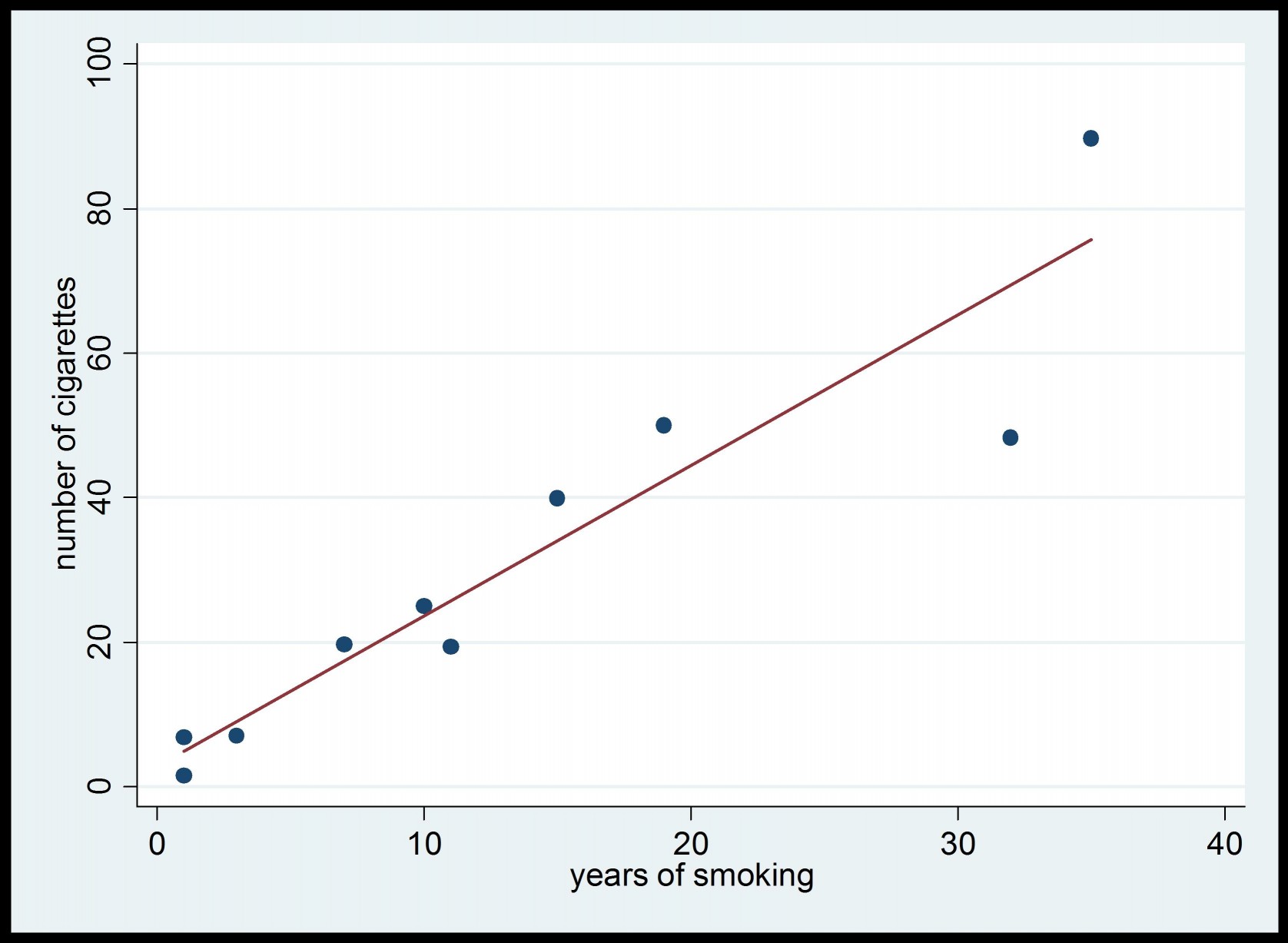
As mentioned earlier, not using the weights in data analysis of complex survey data can seriously bias the results of the analysis, leading to erroneous conclusions. We now illustrate the problem using, again, the tobacco survey as an example. Let us assume that the population $U$ for this study contains 40 persons: 20 men and 20 women. We select a sample $s$ of size 10 using a stratified SRS: 3 men are selected from the men stratum, and 7 women are selected from the women stratum. The aim of the survey is to measure the increase of the number of cigarettes smoked during the day ( $y$ ) with the number of years of smoking ( $x$ ). In other words, we are interested in estimating the regression coefficient $\beta$ . For each of the 10 persons in sample $s$ , the variables $x_k$ and $y_k$ , $k=1,\HDOTS,10 ,$ are measured.

Using the data from the complete population, we are able to compute the true value of the regression coefficient $\beta=\frac{\sum_{k\in U}(Y_k-\overline{Y})(x_k-\overline{X})}{\sum_{k\in U}(x_k-\overline{X})^2}$ , which is equal to 1.88. The data are displayed in Figure 1 below.

Figure 1: Population data from Tobacco Survey

If we separate men and women, we find out that their behaviours are different. For the men, we compute a regression coefficient $\beta_{Men}=\frac{\sum_{k\in U}I_{Men,k}(y_k-\overline{Y}_{Men})(x_k-\overline{X}_{Men})}{\sum_{k\in U}I_{Men,k}(x_k-\overline{X}_{Men})^2}$ of 1.25, and for the women, we obtain $\beta_{Women}$ equal to 2.55. As we can see, women tend to increase their number of cigarettes smoked in a day with the number of years of smoking more than men. This is illustrated in Figure 2 below.

Figure 2: Population Data from Tobacco Survey for Men and Women

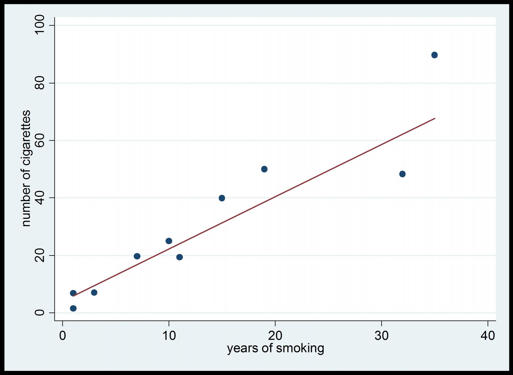
Now, in practice, we do not have data for the complete population, and this is why a survey is conducted. Using the data obtained from the sample $s$ of size 10, we first estimate the regression coefficient $\beta$ using the unweighted estimator $\tilde{\beta}$ given by (4), and we obtain the estimated value 2.08. This is illustrated in Figure 3 below.

Figure 3: Survey Data from Tobacco Survey (unweighted estimator of $\beta$ )

Even after accounting for errors due to sampling, the value of $\tilde{\beta}$ =2.08 is relatively far from the true value $\beta$ . The problem with the computation of the estimate $\tilde{\beta}$ is the fact that the men are under-represented in the sample $s$ , in comparison to women. Although the population $U$ contains the same number of men and women, there are more women in the sample s than men. Given that the smoking behaviour of the women and men are different, the estimate $\tilde{\beta}$ tends to be shifted toward the value of $\beta_{Women}$ . Actually, the estimator $\tilde{\beta}$ is biased with respect to the sampling design. Now, let us estimate the regression coefficient $\beta$ using the weighted estimator $\hat{\beta}$ given by (2). This gives the estimated value 1.82. This is displayed in Figure 4 below.

Figure 4: Survey Data from Tobacco Survey (weighted estimator of $\beta$ .)

As we can see, the value of $\hat{\beta}$ =1.82 is closer to the true value $\beta$ =1.88 than to $\tilde{\beta}$ =2.08. Using an estimator that uses weights, we re-established in the estimator the proportion of men and women that we have in the population. Consequently, although the men are under-represented in the sample $s$ , the weights $w_k$ corrected this under-representation in the computation of the estimate of $\beta$ . Actually, as opposed to $\tilde{\beta}$ , the estimator $\hat{\beta}$ . is almost unbiased (actually, asymptotically unbiased) with respect to the sampling design. Using weighted estimators leads to a better analysis of complex survey data.

It should be noted that if the sampling design is self-weighted, using weighted or unweighted estimators gives the same results. For the tobacco survey, given that the population sizes of men and women are both 10, the sample sizes would then simply need to be the same between men and women. That is, for a total sample size of 10, the sample s should contain 5 men and 5 women to get a self-weighted design.

Now, some statistical analysts claim that they should not use the weights because they are interested in estimating the parameter B of model (3), rather than the finite population quantity $\beta$ . They argue that the sampling design is irrelevant for estimating B, as the weights are functions of the selection probabilities used to select the sample s, and they are not related to the model . If the sampling design does not bring any more information in trying to estimate B, then their claim of not using the weights is true. We then say that the sampling design is not informative. Sampling designs for surveys are informative when the selection probabilities are correlated with the variables of interest, even after conditioning on explanatory variables (e.g., Eideh and Nathan, 2006).

In the case of the tobacco survey, the sampling design is clearly informative, as we see that the smoking behaviour of men is different from the one of women. Having selected more women than men, even if their respective population sizes are the same, influenced the estimation of the regression coefficient. This means that the weights bring some information that is not contained in the model (3). Therefore, in some sense, the model is not “perfect” in trying to explain the relationship between the number of cigarettes smoked during the day and the number of years of smoking. In other words, the model has been misspecified. To correct for this misspecification, the analyst should introduce a gender parameter in model (3) to correctly estimate the regression coefficient of interest.

To prevent model misspecification, in order to obtain good estimates of the parameters of interest, the statistical analyst should use the weights in all situations when dealing with complex survey data. If the sampling design is not informative, using the weights or not should not introduce any significant differences in the estimates if the sample size is not too small. That is, we should have $\tilde{\beta} \approx\hat{\beta}$ . However, if the sampling design turns out to be informative, the weighted estimators $\hat{\beta}$ will produce “better” estimates that will be nearly unbiased and design-consistent.

4. Standard Weighting Steps

As mentioned earlier, the weighting process usually involves three steps. The first step is to obtain design weights (or sampling weights), which are the weights that account for sample selection. The adjustment of the design weights for nonresponse is the second step of the weighting process. Third, the weights are adjusted to some known population totals, which is called calibration. We now describe these three steps in detail.

4.1 Design Weighting

Let $\pi_k=P(k\in s)$ be the probability that population unit $k$ is selected in the sample $s$ . We assume that $\pi_k>0$ for all units $k$ of the population $U$ . That is, all population units have a non-zero chance of being selected in the sample $s$ . For example, with the SRS of 25 individuals from 100, we have $\pi_k=n/N=25/100=1/4$ for all $k\in U$ . The use of unequal probabilities of selection is common in sample surveys. For instance, when a size measure is available for all population units, the population can be stratified and units in different strata may be assigned different selection probabilities. Another possibility is to select the sample with probabilities proportional to the size measure. These unequal probabilities of selection must be accounted for when estimating population parameters; otherwise, bias may result. The most basic estimator of $Y$ that accounts for unequal probabilities of selection is the Horvitz-Thompson estimator (Horvitz and Thompson, 1952), also called the expansion estimator:

(5) $\begin{equation*} \hat{Y}^{HT}=\sum_{k\in s}\frac{y_k}{\pi_k}=\sum_{k\in U}\frac{y_k}{\pi_k}t_k, \end{equation*}$

where $t_k$ is the sample selection indicator variable such that $t_k=1$ if $k\in s$ , and $t_k=0$ , otherwise. The estimator $\hat{Y}^{HT}$ is design-unbiased (or p-unbiased) for $Y$ in the sense that $E_p (\hat{Y}^{HT})=Y$ . The subscript $p$ indicates that the expectation is evaluated with respect to the sampling design. Note that only the sample selection indicators $t_k$ , $k\in U$ , are treated as random when taking a design expectation. The property of $\hat{Y}^{HT}$ to be design-unbiased can be shown by noting that

(6) $\begin{equation*} E_p(t_k)=1\times P(k\in s)+0 \times P(k\notin s)= P(k\in s)=\pi_k. \end{equation*}$

The Horvitz-Thompson estimator $\hat{Y}^{HT}$ , given by (5), can be rewritten as

(7) $\begin{equation*} \hat{Y}^{HT}=\sum_{k\in s}d_k y_k, \end{equation*}$

where $d_k=1/\pi_k$ is the design weight of sample unit $k$ , also called the sampling weight. In this set-up, the design weight $d_k=1/\pi_k$ of unit $k$ can be used as an estimation weight in the absence of nonresponse. The design weight of unit $k$ may be interpreted as the number of units from population $U$ represented by this sample unit. In our previous example, each individual has one chance out of four ( $\pi_k=1/4$ ) of being part of the sample and, therefore, each individual has a design weight of 4. Note that this interpretation is not always appropriate. For instance, consider a population of 100 units with one unit having its selection probability equal to 1/1000 and therefore its design weight equals to 1000. Note also that the design weight does not need to be an integer.

To learn more about sampling theory, the reader may consult books such as Cochran (1977), Grosbras (1986), Särndal et al. (1992), Morin (1993), Tillé (2001), Thompson (2002), Ardilly (2006) and Lohr (2009). It should be noted that Hidiroglou et al. (1995) also present a good overview of weighting in the context of business surveys.

Before discussing how to adjust design weights to account for nonresponse, we first describe the calibration technique.

4.2 Calibration

Calibration arises from a generalisation by Deville (1988), and then by Deville and Särndal (1992), of an idea by Lemel (1976). It uses auxiliary information to improve the quality of design-weighted estimates. An auxiliary variable $x$ , also called a calibration variable, must have the following two characteristics to be considered in calibration:

(i) It must be available for all sample units $k\in s$ ; and

(ii) Its population total $X=\sum_{k\in U}x_k$ must be known.

Often, a vector of auxiliary variables $\mathbf{x}$ is available along with its associated vector of population totals $\mathbf{X}=\sum_{k\in U}\mathbf{x}_k$ . The vector of known population totals can be obtained from the sampling frame, an administrative file or a (projected) census. In practice, the vector $\mathbf{X}$ may be subject to errors, but we assume that they are small enough to be ignored. Examples of auxiliary variables are the revenue of a business or the age group of a person.

The main issue with the use of design weights $d_k$ is that they may lead to confusion since $\hat{\mathbf{X}}^{HT}=\sum_{k\in s}d_k \mathbf{x}_k$ , may not be equal to $\mathbf{X}$ . Calibration fixes this inequality by incorporating auxiliary information in the estimator. It consists of determining calibration weights $w_k^{Cal}$ that are as close as possible to the initial design weights $d_k$ while satisfying the following calibration equation:

(8) $\begin{equation*} \hat{\mathbf{X}}^{Cal}=\sum_{k\in s} w_k^{Cal}\mathbf{x}_k=\sum_{k\in U} \mathbf{x}_k=\mathbf{X} \end{equation*}$

The resulting calibration estimator is denoted by $\hat{Y}^{Cal}=\sum_{k \in s}w_k^{Cal}y_k$ .

Calibration is not only used to remove inconsistencies but also to reduce the design variance of the Horvitz-Thompson estimator $\hat{Y}^{HT}$ . The latter is expected to hold when the calibration variables are correlated with the variable of interest $y$ . To understand this point, let us take an extreme example and suppose that there is a perfect linear relationship between $y$ and $\mathbf{x}$ ; i.e., $y_k=\mathbf{x}^T\boldsymbol{\beta}$ , for some vector $\boldsymbol{\beta}$ . Then, it is straightforward to show that

$\hat{Y}^{Cal}=\sum_{k \in s}w_k^{Cal}y_k=\left(\sum_{k \in s}w_k^{Cal}\mathbf{x}^T_k\right)\boldsymbol{\beta}=\left(\sum_{k \in U}\mathbf{x}^T_k\right)\boldsymbol{\beta}=\left(\sum_{k \in U}y_k\right)=Y.$

In this case, the calibration estimator is perfect; i.e., $\hat{Y}^{Cal}=Y$ with a variance of zero. In general, a perfect linear relationship between $y$ and $\mathbf{x}$ is unlikely and, thus, $\hat{Y}^{Cal}\neq Y$ . However, we may expect that the calibration estimator $\hat{Y}^{Cal}$ will be more efficient than $\hat{Y}^{HT}=Y$ if there is a strong linear relationship between $y$ and $\mathbf{x}$ . Note that calibration can also be used in practice to reduce coverage and nonresponse errors. Again, a linear relationship between $y$ and $\mathbf{x}$ is required to achieve these goals.

More formally, calibration consists of determining calibration weights $w_k^{Cal}$ , for $k\in s$ , so as to minimise

(9) $\begin{equation*} \sum_{k\in s}G_k(w_k^{Cal},d_k) \end{equation*}$

subject to the constraint (8). Deville and Särndal (1992) required that the distance function $G_k(a,b)$ between $a$ and $b$ be such that: (i) $G_k(a,b)\geq 0$ ; (ii) $G_k(a,b)$ is differentiable with respect to $a$ ; (iii) $G_k(a,b)$ is strictly convex; (iv) $G_k(a,b)$ is defined on an interval $\Upsilon_k(b)$ dependent on $k$ and containing $b;$ (v) $G_k(a,a)=0$ ; (vi) $g_k(a,b)=\partial G_k(a,b)\partial a$ is continuous and forms a one-to-one relationship between $\Upsilon_k(b)$ and its image $Im_k(b)$ . It then follows that $g_k(a,b)$ is strictly increasing with respect to a, and that $g_k(a,a)=0$ . Deville and Särndal (1992) gave several examples of distance functions.

Using the method of Lagrange, the minimisation of (9) under the constraint (8) leads to the calibration weight

(10) $\begin{equation*} w_k^{Cal}=d_kF_k(\mathbf{x}_k^T\boldsymbol{\lambda}), \end{equation*}$

where the function $d_k F_k(.)$ is the reciprocal of $g_k(.,d_k)$ that maps $Im_k(d_k)$ onto . The vector $\boldsymbol{\lambda}$ is the vector of Lagrange multipliers. It is obtained as the solution to the equation $\mathbf{X}=\sum_{k \in s}d_k F_k(\mathbf{x}_k^T\boldsymbol{\lambda})\mathbf{x}_k$ , which typically requires an iterative algorithm. Note that $F_k(\mathbf{x}_k^T\boldsymbol{\lambda})$ corresponds to the so-called g-weight from Särndal et al. (1992).

The most popular distance function in practice is the chi-square distance

$G_k(w_k^{Cal},d_k)=\frac{1}{2}\frac{( w_k^{Cal}-d_k )^2}{q_k d_k},$

where $q_k$ is a known constant giving the importance of each unit in the function to be minimised. The choice $q_k=1$ dominates in practice, except when the ratio estimator is used (see below). With this distance function, we obtain

(11) $\begin{equation*} F_k(\mathbf{x}_k^T\boldsymbol{\lambda})=1+q_k \mathbf{x}_k^T\boldsymbol{\lambda}, \end{equation*}$

and the calibration weight has the closed form

(12) $\begin{equation*} w_k^{Cal}=d_k(1+q_k \mathbf{x}_k^T\boldsymbol{\lambda}), \end{equation*}$

with $\boldsymbol{\lambda}=(\sum d_k\mathbf{x}\mathbf{x}^T)^-(\mathbf{X}-\hat{\mathbf{X}^{HT}})$ . For a given square matrix $\mathbf{A}$ , the matrix $\mathbf{A}^-$ is the generalised inverse of $\mathbf{A}$ . Recall that the generalised inverse of $\mathbf{A}$ is any matrix $\mathbf{A}^-$ satisfying $\mathbf{A}\mathbf{A}^-\mathbf{A}=\mathbf{A}$ (Searle, 1971). If the matrix $\mathbf{A}$ is non-singular, then $\mathbf{A}^-$ is unique, and furthermore $\mathbf{A}^-=\mathbf{A}^{-1}$ , the inverse of $\mathbf{A}$ . The resulting calibration estimator is the generalised regression estimator, denoted by $\hat{Y}^{GReg}$ . It can be expressed as

(13) $\begin{equation*} \hat{Y}^{Cal}=\sum_{k \in s}w_k^{Cal}Y_k= \hat{Y}^{HT}+(\mathbf{X}-\hat{\mathbf{X}}^{HT})^T\hat{\boldsymbol{\beta}}=\hat{Y}^{GReg} \end{equation*}$

where $\hat{\boldsymbol{\beta}}=(\sum_{k\in s}q_k d_k\mathbf{x}_k \mathbf{x}_k^T)^{-}\sum_{k\in s}q_k d_k\mathbf{x}_k y_k$ .

The generalised regression estimator has many important special cases (e.g., Estevao et al., 1995). In several surveys, and especially for business surveys, the ratio estimator is often used when there is a single auxiliary variable x. It is obtained by setting $q_k=1/x_k$ . This leads to the calibration weight $w_k^{Cal}=d_k(X/\hat{X}^{HT})$ and the calibration estimator $\hat{Y}^{Cal}=X(\hat{Y}^{Cal}/\hat{X}^{Cal})$ . The ratio estimator is efficient if the relationship between y and x goes through the origin. The well-known Hájek estimator is itself a special case of the ratio estimator when $x_k=1$ , for $k\in U$ . It is written as $\hat{Y}^{Cal}=N(\hat{Y}^{HT}/\hat{N}^{HT})$ , where $\hat{N}^{HT}=\sum_{k\in s}d_k$ .

The post-stratified estimator is another important special case of the generalised regression estimator. It is used when a single categorical calibration variable is available and defines mutually exclusive subgroups of the population, called post-strata. Examples of post-strata are geographical regions or age categories. Let $\delta_{hk}=1$ if unit $k$ belongs to post-stratum $h$ , and $\delta_{hk}=0$ otherwise, for $h=1,\hdots,H$ , with $H$ denoting the total number of post-strata. The post-stratified estimator is a special case of the generalised regression estimator obtained by setting $\mathbf{x}_k^T=(\delta_{1k},\hdots,\delta_{hk})$ and $q_k=1$ . For instance, suppose there are $H=3$ post-strata (three age categories, for example) and that unit k belongs to the second post-stratum. Then, we have $\bold{x}_k^T (0,1,0)$ . The calibration equations are given by

$\sum_{k \in s} w_k^{Cal}\delta_{hk}=\sum_{k \in s_k} w_k^{Cal}=N_h, \quad h=1,\hdots,H,$

where $s_h$ is the set of sample units falling into post-stratum $h$ and $N_h$ is the population count for post-stratum $h$ . The calibration weight of unit $k$ in post-stratum $h$ is given by $w_k^{Cal}=d_k(N_h/\hat{N}_h^{HT})$ , where $\hat{N}^{HT}_h=\sum_{k\in s_h}d_k$ . The calibration estimator reduces to

$\hat{Y}^{Cal}=\sum_{k\in s}w_k^{Cal}y_k=\sum_{h=1}^H \frac{N_h}{\hat{N}^{HT}_h}\sum_{k\in s_h}d_k y_k.$

The above post-stratified estimator reduces to the Hájek estimator when there is only one post-stratum ( $H=1$ ).

Sometimes, two or more categorical calibration variables are available. Post-strata could be defined by crossing all these variables together. However, some resulting post-strata could have quite a small sample size or could even contain no sample units, which is not a desirable property. In addition, the population count of post-strata may not be known even though the population count of each margin is known. Then, only calibration to the known marginal counts is feasible. Raking ratio estimation can then be used in this scenario, which is quite common in social surveys. The reader is referred to Deville et al. (1993) for greater detail on raking ratio estimation.

Calibration estimators have some desirable properties. Indeed, Deville and Särndal (1992) proved that for all $F_k(.)$ satisfying some mild conditions, the calibration estimator $\hat{Y}^{Cal}=\sum_{k \in s}w_k^{Cal}y_k$ , with $w_k^{Cal}$ given by (10), is asymptotically equivalent to the generalised regression estimator $\hat{Y}^{GReg}$ given by (13) since $N^{-1}(\hat{Y}^{Cal}-\hat{Y}^{GReg})=O_p(n^{-1}).$ This can be rewritten as

$N^{-1}(\hat{Y}^{Cal}-Y)= N^{-1}(\hat{Y}^{GReg}-Y)+ O_p(n^{-1})$

Under regularity conditions, $N^{-1}(\hat{Y}^{GReg}-Y)= O_p(n^{-1/2})$ and, thus, $\hat{Y}^{GReg}$ is design-consistent. It follows that $\hat{Y}^{Cal}$ is also design-consistent with the same asymptotic design variance as $\hat{Y}^{GReg}$ . This means that although many distance functions are possible, they all lead to the same asymptotic variance as the one obtained using the chi-square distance.

4.3 Nonresponse Weighting Adjustment

Most surveys, if not all, suffer from nonresponse. Two types of nonresponse can be distinguished: item nonresponse and unit nonresponse. Item nonresponse occurs when information is collected for some but not all the survey variables. Item nonresponse is often treated through imputation, which is outside the scope of this paper. In the following, we will assume that no sample unit is subject to item nonresponse. Unit nonresponse occurs when no usable information has been collected for all the survey variables. It is typically handled by deleting the nonrespondents from the survey data file and by adjusting the design weight of respondents to compensate for the deletions. The resulting nonresponse-adjusted weights can then be calibrated, if some population totals are known.

The main issue with nonresponse is the bias that is introduced when the respondents have characteristics different from the nonrespondents. Also, an additional component of variance is added due to the observed sample size being smaller than the initially planned sample size n. The key to reduce both nonresponse bias and variance is to use nonresponse weighting methods that take advantage of auxiliary information available for both respondents and nonrespondents.

Let us denote by $s_r$ , the set of respondents. That is, the subset of $s$ containing all units for which we were able to measure the variable of interest $t$ . The set of respondents $s_r$ is generated from $s$ according to an unknown nonresponse mechanism $\phi(s_r|s)$ . The response probability $p_k=P(k\in s_r|s,\,k\in s)$ is assumed strictly greater than zero for all $k\in s$ . Nonresponse can be viewed as a second phase of sampling (e.g., Särndal and Swensson, 1987) with the exception that the nonresponse mechanism $\phi(s_r|s)$ is unknown, unlike the second-phase sample selection mechanism in a two-phase sampling design. If the response probability could be known for all $k\in s_r$ ., the double expansion estimator of $Y$ could be used:

(14) $\begin{equation*} \hat{Y}^{DE}=\sum_{k\in s_r} \tilde{d}_k y_k \end{equation*}$

where $\tilde {d}_k=(1/\pi_k)(1/p_k)=d_k/p_k$ is the adjusted design weight. The double expansion estimator is for $Y$ in the sense that $E_{p\phi}(\hat{Y}^{DE})=Y$ . This follows from $E_{\phi}\left(\hat{Y}^{DE}\vert s\right)=\hat{Y}^{HT}$ and the design unbiasedness of $\hat{Y}^{HT}$ as an estimator of $Y$ . The subscript $\phi$ indicates that the expectation is evaluated with respect to the nonresponse mechanism.

The response probability $p_k$ is unknown in practice unlike the second-phase selection probability in a two-phase sampling design. To circumvent this difficulty, the response probability $p_k$ can be estimated using a nonresponse model. A nonresponse model is a set of assumptions about the multivariate distribution of the response indicators $r_k$ , $k\in s$ . The estimated response probability of unit $k$ is denoted by $\hat{p}_k$ and the nonresponse-adjusted design weight by $\hat{d}_k=d_k/\hat{p_k}$ . The resulting nonresponse-adjusted estimator is $\hat{Y}^{NA}=\sum_{k\in s}\hat{d}_k y_k.$ . It is typically not $p\phi$ -unbiased anymore but, under certain conditions, it is at least $p\phi$ –constisitent. Most methods for handling nonresponse simply differ in the way the response probability is estimated. In the rest of this section, we focus on the modeling and estimation of $p_k$ .

Ideally, the expanded variable $\breve{y}_k=d_k y_k$ would be considered as an explanatory variable in the response probability model. In other words, the response probability would be defined as $p_k\equiv P(r_k=1|s, k\in s,\breve{Y_k})$ , $k\in s$ . As pointed out above, this would ensure that the double expansion estimator $\hat{Y}^{DE}$ is $p\phi$ –unbiased. Note that if there are many domains and variables of interest, the number of potential explanatory variables could become quite large. Unfortunately, $\breve{y}_k$ is not known for the nonrespondents, $k\in s-s_r$ , and can thus not be used as an explanatory variable. The most commonly-used approach to deal with this issue is to replace the unknown $\breve{y}_k$ by a vector $\bold{z}_k$ of explanatory variables available for all sample units $k\in s$ . The vector $\bold{z}_k$ must be associated with the response indicator $r_k$ . Ideally, it must also be associated with $\breve{y}_k$ , as it is a substitute for $\breve{y}_k$ . This is in line with the recommendation of Beaumont (2005) and Little and Vartivarian (2005) that explanatory variables used to model nonresponse should be associated with both the response indicator and the variables of interest.

Explanatory variables that are not associated with the (expanded) variables of interest do not reduce the nonresponse bias and may likely increase the nonresponse variance. Explanatory variables can come from the sampling frame, an administrative file and can even be paradata. Paradata, such as the number of attempts made to contact a sample unit, are typically associated with nonresponse but may or may not be associated with the variables of interest. Therefore, such variables should not be blindly incorporated into the nonresponse model (Beaumont, 2005).

The use of $\mathbf{z}_k$ as a replacement for $\breve{y}_k$ implies that the response probability is now defined as $p_k\equiv P(r_k=1\vert s, k\in s, \mathbf{z}_k)$ . The double expansion estimator (14) remains $p\phi$ -unbiased, if the following condition holds:

(15) $\begin{equation*} P(r_k=1\vert s, k\in s, \mathbf{z}_k,\breve{y_k})= P(r_k=1\vert s, k\in s, \mathbf{z}_k)\equiv p_k. \end{equation*}$

Condition (15) implies that the nonresponse mechanism does not depend on any unobserved value and, thus, that the values of the variable of interest are missing at random (Rubin, 1976). In addition to condition (15), it is typically assumed that sample units respond independently of one another. In order to obtain an estimate of $p_k$ , one may consider a parametric model. A simple parametric response probability model is the logistic regression model (e.g., Ekholm and Laaksonen, 1991):

(16) $\begin{equation*} p_k=p(\mathbf{z}_k;\boldsymbol{\alpha})=\frac{1}{1+exp(-\mathbf{z}_k^T\boldsymbol{\alpha})}. \end{equation*}$

here $\boldsymbol{\alpha}$ is a vector of unknown model parameters that needs to be estimated. If we denote by $\hat{\boldsymbol{\alpha}}$ , an estimator of $\boldsymbol{\alpha}$ then the estimated response probability is given by $\hat{p}_k^{LR}=p(\mathbf{z}_k;\hat{\boldsymbol{\alpha}})$ . The logistic function (16) ensures that $0<\hat{p}_k^{LR}<1$ . The maximum likelihood method can be used for the estimation of $\boldsymbol{\alpha}$ .

Calibration may also be directly used to adjust for the nonresponse. This is the view taken by Fuller et al. (1994), Lundström and Särndal (1999) and Särndal and Lundström (2005), among others. There is a close connection between calibration and weighting by the inverse of estimated response probabilities. However, we prefer the latter view because it states explicitly the underlying assumptions required for the $p\phi$ -consistency of $\hat{Y}^{NA}$ as an estimator of the population total $Y$ , such as assumptions (15) and (16). In addition, it stresses the importance of a careful modeling of the response probabilities. Once nonresponse-adjusted weights $\hat{d}_k$ have been obtained, nothing precludes using calibration to improve them further. That is, we may want to determine the calibration weights $\hat{w}_k^{Cal}$ , $k\in s_r$ , that minimise $\sum_{k\in s_r}G_k(\hat{w}_k^{Cal},\hat{d}_k)$ subject to the constraint $\sum_{k\in s_r}\hat{w}_k^{Cal}\mathbf{x}_k=\mathbf{X}$ . This is a problem very similar to the one discussed in Section 4.2.

There are two main issues with using the logistic regression model (16): (i) it may not be appropriate, even though careful model validation has been made; (ii) it has a tendency to produce very small values of $\hat{p}_k$ yielding large weight adjustments $1/\hat{p}_k$ . The latter may cause instability in the nonresponse-adjusted estimator $\hat{Y}^{NA}$ . A possible solution to these issues is obtained through the creation of classes that are homogeneous with respect to the response propensity. Ideally, every unit in a class should have the same true response probability. The score method (e.g., Little, 1986; Eltinge and Yansaneh, 1997; or Haziza and Beaumont, 2007) attempts to form these homogeneous classes. Forming homogeneous classes provides some robustness to nonresponse model misspecifications and is less prone to extreme weight adjustments than using $1/\hat{p}_k^{LR}$ . There are other methods than the score method, such as the CHi-square Automatic Interaction Detection (CHAID) algorithm developed by Kass (1980). In stratified business surveys, classes are sometimes taken to be the strata for simplicity and because there may be no other explanatory variables available.

4.4 Practical Issues

In addition to nonresponse and calibration, weights can be adjusted for other reasons. First, we might be interested in adjusting the set of weights $\{w_k; k\in s\}$ globally to account for under- or over-coverage of the population $U$ . In this case, we assume that by some means (a census, administrative data, etc.) we know the true size $N^*$ of the target population, which turns out to be different from the size $N$ of the sampling frame. We then adjust the weights $w_k$ so that they no longer sum to $N$ , but rather to $N^*$ . One way to achieve this is by calibrating (or post-stratifying) on $N^*$ .

We might also be interested in adjusting the weights of some particular units only. One reason for this can be that the value of the variable of interest y is found to be an outlier. Outliers are values that are atypical compared to the other values of the population. Usually, an outlier is detected by searching for extreme large values in the sample (or in the population). The effect of a unit $k^'$ being an outlier in a sample is to produce abnormally large estimates of totals $\hat{Y}=\sum_{k\in s}w_k y_k$ . Although the outlying value of $y_{k^'}$ within the sample $s$ can be a true value, the statistician might not believe that there are $w_{k^'}$ -1 other units in the population that have similar values to $y_{k^'}$ . In other words, it is felt that weight $w_{k^'}$ does not correspond to the number of units from the population that are represented by the sample unit $k^'$ . For this reason, the weight of unit $k^'$ . is then trimmed, and in practice this reduction is often set to 1 (e.g., Potter, 1990). This means that for the outlying unit $k^'$ ., we set its weight to $\tilde{w}_{k^'}$ =1, and we adjust the other weights so that $\sum_{k\in s}\tilde{w}_{k}=\tilde{w}_{k^{'}}+\sum_{k\in s, k \neq k^{'} }\tilde{w}_{k}=N$ . The total $Y$ is then estimated using $\tilde{Y}=\sum_{k\in s}\tilde{w}_k y_k$ , which aims to produce a “better” estimate than the original estimate . The effect of weight trimming has often a limited impact on the design variance of the Horvitz-Thompson estimator. See Beaumont and Rivest (2009) for more on this subject. Note that by adjusting the weights for outliers, we are introducing a bias in the estimates, but it is hoped that this bias will be small compared to the gain of precision obtained.

There are several other reasons why the survey statistician might want to adjust the sampling weights: an outdated sampling frame, duplication of units within the frame, subject-matter knowledge, etc.

5. Conclusion

After giving some context about weighting in sample surveys, we explained why we should use weights in statistical analysis of complex survey data. We concluded that in order to obtain good estimates of the parameters of interest, the statistical analyst should use the weights in all situations when dealing with complex survey data. If the sampling design is not informative, using the weights or not should not introduce any significant differences in the estimates. However, if the sampling design turns out to be informative, the use of weighted estimators will produce “better” results.

We also described the weighting process, which involves three steps. The first step is to obtain design weights. The second step of the weighting process is the adjustment of the design weights for nonresponse. Third, the weights are calibrated to some known population totals.

It is hoped that the reader has understood the importance of weights, not only in the production of finite population statistics, but also in the statistical analysis of survey data. As well, by giving some notions on how the weights are usually computed, we wanted the reader to understand better what weights represent.

References

Ardilly, P. (2006). Les techniques de sondage, 2ème édition. Éditions Technip, Paris, 696 pages.
Beaumont, J.-F. (2005). On the use of data collection process information for the treatment of unit nonreponse through weight adjustment. Survey Methodology, 31, 227-231.
Beaumont, J.-F., Rivest, L.-P. (2009). Dealing with outliers in survey data. In Handbook of Statistics, Sample Surveys: Theory, Methods and Inference, Vol. 29, Chapter 11, Ed. D. Pfeffermann and C.R. Rao, Elsevier BV.
Binder, D.A. (1983). On the variances of asymptotically normal estimators from complex surveys, International Statistical Review, 51, 279–292.
Chambers, R.L., Skinner, C.J. (Eds.) (2003). Analysis of Survey Data, John Wiley & Sons, New York.
Cochran, W.G. (1977). Sampling Techniques, third edition. John Wiley and Sons, New York, 428 pages.
Deville, J.-C. (1988). Estimation linéaire et redressement sur information auxiliaires d’enquêtes par sondage. In Essais en l’honneur d’Edmond Malinvaud (Eds. A. Monfort and J.J. Laffont), Economica, Paris, pp. 915-927.
Deville, J.-C., Särndal, C.-E. (1992). Calibration estimators in survey sampling. Journal of the American Statistical Association, Vol. 87, No. 418, June 1992, pp. 376-382.
Deville, J.-C., Särndal, C.-E., Sautory, O. (1993). Generalized raking procedures in survey sampling. Journal of the American Statistical Association, 88, 1013-1020.
Eideh, A. H., Nathan, G. (2006). The Analysis of Data from Sample Surveys under Informative Sampling. Acta et Commentationes Universitatis Tartuensis de Mathematica, Tartu 2006, Volume 10, pp 41-51.
Ekholm, A., Laaksonen, S. (1991). Weighting via response modeling in the Finnish Household Budget Survey. Journal of Official Statistics, 7, 325–337.
Eltinge, J. L., Yansaneh, I. S. (1997). Diagnostics for formation of nonresponse adjustment cells, with an application to income nonresponse in the U.S. Consumer Expenditure Survey. Survey Methodology, 23, 33-40.
Estevao, V.M., Hidiroglou, M.A., Särndal, C.-E. (1995). Methodological principles for a generalized estimation system at Statistics Canada. Journal of Official Statistics, 11, 2, 181-204.
Fuller, W.A., Loughin, M.M., Baker, H.D. (1994). Regression weighting in the presence of nonresponse with application to the 1987-1988 Nationwide Food Consumption Survey. Survey Methodology, 20, 75-85.
Grosbras, J.-M. (1986). Méthodes statistiques des sondages. Economica, Paris.
Haziza, D., Beaumont, J-F (2007). On the construction of imputation classes in surveys. International Statistical Review, 75, 25-43.
Hidiroglou, M.A., Särndal, C.-E., Binder, D.A. (1995). Weighting and estimation in business surveys. In Business Survey Methods (Eds. Cox, Binder, Chinnappa, Christianson, Colledge and Kott), John Wiley and Sons, New York, 732 pages.
Horvitz, D.G., Thompson, D.J. (1952). A generalization of sampling without replacement from a finite universe. Journal of the American Statistical Association, Vol. 47, pp 663-685.
Korn, E.L., Graubard, B.I. (1999). Analysis of Health Surveys, John Wiley & Sons, New York.
Kass, V.G. (1980). An exploratory technique for investigating large quantities of categorical data. Journal of the Royal Statistical Society, Series C (Applied Statistics), 29, 119-127.
Lemel, Y. (1976). Une généralisation de la méthode du quotient pour le redressement des enquêtes par sondage. Annales de l’INSEE, Vol. 22-23, pp. 272-282.
Li, J., Valliant, R. (2009). Survey weighted hat matrix and leverages, Survey Methodology, 35(1), 15–24.
Little, R. J. A. (1986). Survey nonresponse adjustments for estimates of means. International Statistical Review, 54, 139-157.
Little, R.J., Vartivarian, S. (2005). Does weighting for nonresponse increase the variance of survey means?, Survey Methodology, 31, 161-168.
Lohr, S. (2009). Sampling: Design and Analysis, 2^nd Edition. Duxbury Press, California, 600 pages.
Lundström, S., Särndal, C.-E. (1999). Calibration as a standard method for the treatment of nonresponse. Journal of Official Statistics, 15, 305-327.
Morin, H. (1993). Théorie de l’échantillonnage. Presses de l’Université Laval, Ste-Foy, 178 pages.
Pfefferman, D., Skinner, C.J., Holmes, D.J., Goldstein, H., Rasbash, J. (1998). Weighting for unequal selection probabilities in multilevel models, Journal of the Royal Statistical Society, Series B 60(1), 23–40.
Potter, F. (1990). A study of procedures to identify and trim extreme sampling weights. In Proceedings of the Section on Survey Research Methods, American Statistical Association, 225-230.
Rao, J.N.K., Scott, A.J. (1981). The analysis of categorical data from complex sample surveys: Chi-squared tests for goodness of fit and independence in two-way tables, Journal of the American Statistical Association, 76, 221–230.
Rao, J.N.K., Wu, C.F.J. (1988). Resampling inference with complex survey data, Journal of the American Statistical Association, 83, 231–241.
Roberts, G., Rao, J.N.K., Kumar, S. (1987). Logistic regression analysis of sample survey data, Biometrika, 74, 1–12, 1987.
Rubin, D.B. (1976). Inference and missing data. Biometrika, 53, 581-592.
Särndal, C.-E, Lundström, S. (2005). Estimation in Surveys with Nonresponse. John Wiley and Sons, West Sussex, England, 200 pages.
Särndal, C.-E., Swensson, B. (1987). A general view of estimation for two-phases of selection with applications to two-phase sampling and nonresponse. International Statistical Review, 55, 279–294.
Särndal, C.-E., Swensson, B., Wretman, J. (1992). Model Assisted Survey Sampling. Springer-Verlag, New York.
Searle, S.R. (1971). Linear Models. John Wiley and Sons, New York, 532 pages.
Stapleton, L.M. (2008). Variance estimation using replication methods in structural equation modeling with complex sample data. Structural Equation Modeling: A Multidisciplinary Journal, 15(5), 183–210.
Thompson, S.K. (2002). Sampling, 2^nd Edition. John Wiley and Sons, New York, 400 pages.
Tillé, Y. (2001). Théorie des sondages – Échantilllonnage et estimation en populations finies. Dunod, Paris, 2001, 284 pages.

Why We Should Put Some Weight on Weights.

Special issue

Abstract

Keywords

Copyright

1. Introduction

2. Weighting in Sample Surveys

3. The Use of Weights in Statistical Analysis

4. Standard Weighting Steps

4.1 Design Weighting

4.2 Calibration

4.3 Nonresponse Weighting Adjustment

4.4 Practical Issues

5. Conclusion

References

Call for papers. Submit till April 30, 2024!

Login

Keywords

Digitize!

FORS

GESIS