Pouring water into wine: revisiting the advantages of the crosswise model for asking sensitive questions

---

Abstract

The Crosswise Model (CM) has been proposed as a method to reduce effects of social desirability in sensitive questions. In contrast with former variants of Randomized Response Techniques (RRTs), the crosswise model neither offers a self-protective response strategy, nor does it require a random device. For these reasons, the crosswise model has received a lot of positive attention in the scientific community. However, previous validation studies have mostly analysed negatively connoted behaviour and thus draw on the principle of “more is better”. Higher prevalence rates of socially undesirable behaviour in the crosswise model cannot be attributed unambiguously to a reduction in social desirability bias, since random ticking resulting from respondent confusion about the question format cannot be ruled out as an alternative explanation. Unlike most research on crosswise models and randomized response techniques, we conduct an experiment in a general population survey that does not assess negatively connoted but socially desirable behaviour (namely, whether respondents had donated blood within the last twelve months). This design allows us to empirically disentangle the reduction of social desirability bias from random responses. We find signifcantly higher prevalence rates in the crosswise condition than in the direct question. What is more, we could not identify any subgroup of respondents, in which the CM successfully reduced social desirability bias. These results cast doubts on the validity of cosswise models. They suggest that a considerable number of respondents do not comply with the intended procedure.

Keywords

crosswise model, randomised response techniques, sensitive questions, social desirability

Acknowledgement

This paper is based on presentations given at the Rational Choice Seminar (Venice) in 2014 and at the ESRA Conference (Reykjavik) in 2015. The project to validate the CM was implemented into a community-based panel survey without any extra resources. We thank Katrin Auspurg as well as Andreas Diekmann, Marc Höglinger, and the other participants of the Rational Choice Seminar for their valuable comments on earlier versions of this paper.

Introduction: Obtaining True Answers to Sensitive Questions

Asking sensitive questions in a way that ensures honest answers and valid inferential estimates is a particularly demanding challenge in survey research. The researchers’ main concern in this context is the avoidance of social desirability bias (SDB) (for an overview see Krumpal 2013; Wolter 2012). Particularly when survey questions touch on private, socially undesirable or even illegal behaviours (Lensvelt-Mulders 2008: 462, Tourangeau and Yan 2007: 860), respondents are usually reluctant to answer truthfully.

According to Paulhus (2002), two different response behaviours can drive SDB: Respondents can either describe themselves as saints (by denying negative attributes) or superheros (by highlighting positive attributes). Paulhus furthermore distinguishes between self-deception and other-deception (or impression management). Self-deception is assumed to be a rather unconscious process that aims to maintain a positive self-image and to reduce cognitive dissonance, while other-deception takes place consciously to obtain social approval and avoid negative consequences. These two aspects of SDB are empirically supported by the results of Holtgraves’ experiments on SDB and latency times (Holtgraves 2004). The author assesses the question to which extent social desirable responding is a conscious or an automatic process, and whether it affects the retrieval process itself (e.g. its thoroughness): Interestingly, heightening social desirability concerns goes hand in hand with longer response times. These results make it plausible that respondents who give socially desirable answers actually engage in a full retrieval process but edit their responses afterwards if necessary. However, the study also identifies a particular group of respondents who apparently performed the editing process with lower effort: Respondents with a disposition to self-deception needed a particularly short time to give socially desirable answers. Empirically, the author cannot exclude the possibility that some respondents might immediately switch into a „pure faking strategy“ (Holtgraves 2004: 171), a widely automatic process, in which the respondent completely omits the retrieval of relevant information. Following these results, socially desirable responding can be an effortless task that is performed very quickly, but mostly seems to be a consciously planned behaviour that requires more time.

Rational choice theory provides a systematic theoretical framework to explain under which circumstances misreporting becomes likely (Esser 1986; Becker 2006) as well as empirical evidence that SDB can be seen as a function of personal approval motive, differences in the perceived desirability of response options, and privacy of the interview situation (Stocké 2007). In line with the rational choice approach, a lot of reasonable advice has been formulated to avoid SDB. This usually includes neutral question wording, ensuring anonymity, non-reactive modes of data collection, or (if these are not possible) well-trained interviewers who avoid giving any sign of judgement (Diekmann 2014; Groves et al. 2009; Lensvelt-Mulders 2008).

Special question formats have, however, also been proposed to assess sensitive questions. A frequently applied approach when asking sensitive questions are randomized response techniques (RRTs). This paper will focus on the crosswise model (CM), a recent RRT variant proposed by Yu, Tian and Tang (2008). This model has been put forward as a way of overcoming some of the flaws RRTs suffers from, because it seems much easier to implement and for respondents to understand. Since it does not require a random device, it is sometimes also called a “nonrandomized response technique”.

This paper empirically evaluates the validity of the CM in a survey experiment on blood donation, which allows us to disentangle the reduction of SDB from random ticking. It arrives at a critical conclusion: although the CM is a straightforward way of masking sensitive topics, respondents still have problems understanding the task and do not always answer truthfully.

 

RRTs: Rise and Fall?

Originally proposed by Warner (1965), numerous RRT implementation variants have been developed over time. All RRT strategies, however, share the common feature that some additional noise is added to the data by means of a random device (like dice or coins) with a known probability distribution. The researcher does not gain any knowledge about the individual answer to the sensitive question, meaning that an answer is no longer revealing and that the respondents’ privacy is ensured. Nonetheless, the individual answer is linked probabilistically to the sensitive behaviour, and a prevalence rate can be estimated at the aggregate level. Regression models adapted for RRTs even provide additional information on how covariates are linked to certain respondent groups’ probability to admit a sensitive behaviour.

Despite their popularity, RRTs suffer from some disadvantages. One is related to the use of random devices, particularly in online applications. Although it is possible in principle to draw random numbers within web surveys, this procedure requires the respondent’s trust insofar as those digits could theoretically be manipulated by the researcher or saved to the obtained data set. Alternatively, respondents can be asked to throw coins or dice. While this strategy might still work well in face-to-face interviews, it is not under the researcher’s control if the respondent goes through this effort when survey completion takes place in a self-administered mode. The participant could just as well pick a number or give arbitrary answers.

Apart from these challenges related to random devices, RRTs not only increase statistical noise and make estimates less precise; they also are cognitively demanding. They require more response time than direct questioning (DQ) and might confuse respondents, trigger mistrust and cause arbitrary or faked responses or nonresponse.

Some studies report considerable rates of respondents who refuse to answer the RRT question (Coutts & Jann 2011:179; van der Heijden et al. 2000:520; Kirchner et al. 2013:298; Krumpal 2012:1393), as well as high cognitive burdens according to respondents‘ self-reports (Coutts & Yann 2011:179; Krumpal 2012:1393,1400; van der Heijden et al. 2000:520) or interviewers’ evaluations (Krumpal & Näher 2012:273) and non-compliance with RRT instructions (Edgell, Himmelfarb, & Duchan 1982; Ostapczuk, Musch, & Moshagen 2011).

In principle, untruthful answers in RRTs can be explained by misunderstandings concerning the rather complicated procedure. A competing explanatory approach might be that respondents do not trust the procedure and therefore intentionally cheat on it. In line with the first theoretical concept, some authors focus on the effects of educational background, age and reported clarity of instructions on response behaviour. Krumpal (2012) reports that older and less educated respondents were overrepresented among the respondents who refused to answer the RRT question in his study. He concludes that “the subgroup of RRT deniers […] seems to be more inclined to misunderstand the principle of RRT and, as a consequence, to develop less trust and cooperation” (Krumpal 2012:1400). This result is to some extent supported by Landsheer, Heijden, and Gils (1999), who suggest that higher reading and writing skills help the respondents develop more trust in the method, which in turn reduces nonresponse rates. Some authors conclude that a higher educational background (Bockenholt & Heijden 2007) or a better understanding of the procedure (van der Heijden et al. 2000) favours more accurate responses, while other studies do not find the expected education effect (Holbrook & Krosnick 2010; Wolter & Preisendörfer 2013).

Support for intentional misreporting can be found in a number of studies that have identified problems with forced answers. More concretely, “innocent” respondents are reluctant to give an answer that could falsely be interpreted as admitting to a socially undesirable behaviour. Particularly in so-called asymmetric RRT variants, in which one of the possible answers directly translates into a statement about a sensitive behaviour (typically because no false NO answers are provoked), respondents tend to play safe by making use of the obvious evasive answering strategy that is never associated with the undesirable behaviour (Coutts & Jann 2011; John et al. 2013; Ostapczuk et al. 2009). However, even for a symmetric implementation with a manipulated random device, Edgell et al. (1982) report that between 4 and 26 percent of respondents ignored RRT instructions if they were directed towards a seemingly embarrassing forced answer. A number of studies also partly report negative prevalence estimates that suggest non-compliance with instructions (Coutts & Jann 2011; John et al. 2013; Kirchner et al. 2013), bringing about inconsistent results when DQ and RRT are compared: the RRT yields less valid estimates than DQ (Coutts et al. 2011; Holbrook & Krosnick 2010 for an experiment on a socially desirable behaviour), or only produces preferable estimates for some of the examined items or subgroups (Kirchner et al. 2013; Locander, Sudman, & Bradburn 1976; Umesh & Peterson 1991; Wolter & Preisendörfer 2013). A growing but still modest number of validation studies with individual level data also suggest that RRT does not solve the problem of underreporting: rather, it brings about unpredictably directed biases and low validity (Edgell et al. 1982; van der Heijden et al. 2000; Höglinger, Jann, & Diekmann 2016; John et al. 2013; Locander et al. 1976; Wolter & Preisendörfer 2013).

In sum, RRTs only sometimes reduce SDB, meaning that it is not clear under what circumstances the approach actually works (for a descriptive summary, see Umesh & Peterson 1991:113 et seq and 122 et seq). Although Lensvelt-Mulders, Hox, van der Heijden, & Maas (2005) conclude that, overall, RRT slightly helps to reduce SDB on the basis of a meta-analysis, the variance in results is remarkable; estimates attained by RRTs are often not comparable, even though they use similar items and samples.

 

The CM: A Validation Study

The CM is a rather new procedure with high hopes for overcoming the problems of traditional RRTs. It consists of two questions, both of which can be answered with “yes” or “no”. The first item is non-sensitive with a known probability; the second refers to the sensitive behaviour of interest. The crucial idea of the model is that respondents do not answer these questions separately, but state only if their answers to both questions are equal or different.

 

Table 1. Basic logic of the CM

 

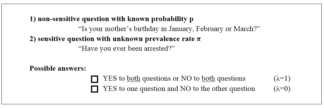
Due to the combination of two “yes” answers and two “no” answers in one category , an individual response to the combined items cannot be linked directly to the sensitive behaviour. Unlike in traditional forms of the RRT, there are no revealing answers or self-protective strategies in CMs. Respondents should be able to understand that it is impossible to trace back their answer, so they can answer honestly without fearing any consequences. The CM is, moreover, easy to implement online or in pen and paper surveys, because it does not make use of a random device.

Despite the privacy protection that comes with the CM, the researcher can calculate a prevalence estimate at the aggregate level. Knowing that the first response category  will be ticked if both items are answered with “yes” or if both items are answered with “no” , the prevalence rate can be estimated for given λ and p by using the following formula:

The CM is formally equivalent to the RRT originally proposed by Warner (1965), who randomly directed respondents either to the original sensitive question (such as “Have you ever been arrested?”) or its negation (such as “Have you never been arrested?”). As RRTs, it sacrifices some statistical precision to protect respondent privacy. Researchers will therefore be particularly interested to know if this trade-off pays off by obtaining more reliable answers from their respondents.

Previous research

A growing number of studies use CMs, covering diverse topics from plagiarism and tax evasion to drug use. When compared to DQ in an experimental setup with student samples, those studies usually find higher prevalence rates for the socially undesirable behaviour in the CM condition (Coutts et al. 2011; Hoffmann et al. 2015; Hoffmann & Musch 2016; Höglinger, Jann, & Diekmann 2014; Jann, Jerke, & Krumpal 2012; Korndörfer, Krumpal, & Schmukle 2014; Kundt 2014; Kundt, Misch, & Nerre 2013; Nakhaee, Pakravan, & Nakhaee 2013; Shamsipour et al. 2014). Since it is generally assumed that higher prevalence rates for socially undesirable behaviour are synonymous with better, less biased measurement, this higher prevalence in the CM have usually been interpreted as a positive sign of the usefulness of the model. This explains why judgements about the CM were very optimistic in the first years after the idea was published, and why the scientific community believed for a while that the CM “offers a valid and useful means for achieving the experimental control of social desirability” (Hoffmann & Musch 2016:11). Only very recently have the first serious validation attempts been undertaken to evaluate this new and promising procedure, and some doubts have been raised about the adequacy of the estimates (Höglinger 2017).

Questioning the assumption that “more is better” for undesirable behaviour with low prevalences

The crucial problem in nearly all CM applications is that they assess undesirable behaviour with low prevalence rates and, as a logical consequence, rely on the assumption that higher prevalence estimates mean better estimates. Unfortunately, this is not necessarily true. It is actually straightforward to show that it is impossible to validate the CMs performance when undesirable behaviour with low prevalence rates is assessed (unless the true individual answers are known).

Respondents might use a heuristic answering strategy to avoid cognitive burden, or they might mistrust the researcher and tick answers randomly.[1] In this case, would tend towards 0.5 – as well as the estimated prevalence rate .

As a matter of fact, we would also expect higher prevalence rates than in DQ if the CM elicited correct values – that is, if it actually reduced SDB. In other words, the CM estimates tend towards the same direction, both if the model works properly and if the respondents tick randomly. Fatally, it is thus impossible to tell if the seemingly promising results are driven by real prevalence rates or by the complicated question format.

What we want to suggest here is an easy approach to disentangle these usually intertwined phenomena: the assumption that “less is better” for socially desirable behaviours with low prevalences. By asking respondents about a rare but socially desirable behaviour, we expect lower prevalence rates if the CM actually reduces SDB, but higher estimates if random ticking drives the results.[2]

Put more generally, a reduction of SDB and heuristic random responses can only be distinguished if those phenomena have different implications for prevalences when compared to DQ formats. As Table 2 shows, this is only the case if socially desirable behaviour with low prevalence rates or deviant behaviour with high prevalence rates is assessed (highlighted in grey). In this latter case, the estimated prevalence rate still tends towards 50 percent if respondents tick response categories randomly. We would therefore expect higher prevalences in the CM condition if the method successfully reduced SDB, but lower estimates if respondents did not follow the instructions.

 

Table 2. Disentangling random ticking and reduction of SDB

 

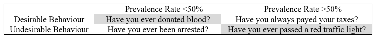
In the remaining cases, including the most common approach of assessing deviant behaviour with low prevalences, higher estimates can undistinguishably result from more accurate answers, as well as from random ticking.

Data and experimental setup

Our validation study has the advantage that it assesses a low prevalence behaviour that is socially desirable, namely blood donation. Relying on the assumption that “less is better”, this approach allows us to evaluate the CM’s potential to reduce SDB without confounding it with effects of random answers due to cognitive overburdening.

The experiment was implemented in the sixth wave of a representative general population panel survey in Konstanz, a town in South Germany. The data collection took place in autumn 2013. Apart from methodological experiments, the questionnaire mainly covered topics like local policies and life satisfaction (for a detailed report, see Hinz, Mozer, & Walzenbach 2014).

The sampling procedure was based on a random selection of registered citizens who were at least 18 years old. Apart from the already existing panel members (N=1,381), a refreshment sample (N=2,770) was newly invited to the sixth wave. In both groups, initial recruitment for the panel took place by means of a postal invitation letter, in which the selected sample is asked to sign up for the annual web survey. Once they registered, the survey was usually issued to the respondents online, or (upon request) as a paper questionnaire.

If we apply a conservative measure (equivalent to the “minimum response rate” or “response rate 1” according to AAPOR standard definitions) treating all cases of unknown eligibility and partially completed questionnaires as unit-nonresponse, the response rate among the already registered panel members was 56.3 percent; among the refreshment sample 20.9 percent could be recruited for survey participation. All in all, this leaves us with 1,037 online and 322 paper questionnaire participations. In terms of sex and age, our sample reflects the distributions we would expect from the town council’s official registry data. Although there is no official information available for educational attainment, the universities in Konstanz surely contribute to a comparatively high education level among the general population (see section I in Appendix for more details).

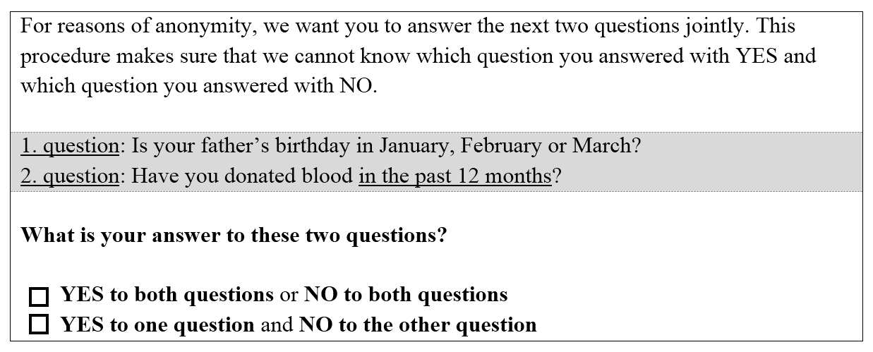
Within each survey mode, respondents were randomly assigned to one of two experimental conditions. To at least partially compensate for the loss of statistical efficiency in RRTs, two thirds were directed to the CM format, one third to the DQ. The CM was briefly explained in an introductory sentence. The participants were then asked to answer the blood donation item jointly with a question about their father’s birthday. Assuming that birthdays are distributed equally over the year, the probability for this item is known, and we can estimate the prevalence rate for blood donation.

 

Table 3. The CM on blood donation

 

In 19 cases, participants refused to answer the blood donation question but continued the questionnaire on the following page. It is worth noting that this kind of item-nonresponse occurred 17 times in the CM condition and twice in the DQ format, which are low numbers with regard to dropout. This left us with 1,340 valid responses that could be used for analysis: 855 from the CM, and 485 from the DQ condition.

Results

Figure 1 compares the shares of respondents who confirmed that they had donated blood in the past twelve months for the two experimental conditions. The result is striking. While 11.1 percent of the respondents confirmed having donated blood when asked with DQ, the share for the group who answered the CM is 18.1 percent. This result is very evidently not in line with what we would expect to see if the CM worked properly. Since “less is better” for socially desirable behaviour in the CM, survey participants should have been more willing to admit that they had not donated blood. However, we see the exact opposite, suggesting that the CM actually deteriorates our prevalence estimates.

 

Figure 1: Prevalence rates obtained by DQ and CM

 

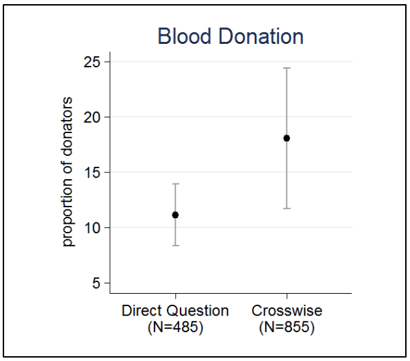
This interpretation is furtherly confirmed by a second validation criterion. Apart from being able to compare results from the DQ and CM, we also have the possibility of estimating the true prevalence by using official data from the Red Cross, which administers all local blood donation campaigns. Hoffmann et al. would call this a strong validation criterion that can only be applied in the rare cases when the true prevalence rate is known, distinguishing it from weak validation criteria which traditionally compare RRT estimates to DQ formats, while relying on the assumption that “more is better” (Hoffmann et al. 2015:404). Dividing the number of blood donations registered in Konstanz in 2012 by the number of inhabitants over 18 at that time yields a prevalence rate of about four percent.[3] In the likely event that some people donated more than once, this estimate would decrease even further. We therefore assume that the true value ranges below four percent. This means that we are radically overestimating the true prevalence rates – both in the DQ format, and (more importantly) even more so in the CM, which should have reduced the number of socially desirable answers.[4]

Why? – Regression analyses

In sum, estimates elicited from DQ suffered from SDB, but those obtained in the CM were even worse. Why? Did respondents misreport intentionally, or were they accidently making mistakes because the question format was not that intuitive after all? Were they deliberately choosing an evasive answering strategy like random ticking to avoid cognitive burden?

To get an idea of the number of inaccurate responses, we calculated the number of respondents who would have to tick answers randomly in the CM condition to obtain the results described above. If we assume a share of random tickers , the number of respondents who comply with the intended procedure is given by . Since random tickers will have a of 0.5 by definition, an estimate for the share of random tickers in our data is easily obtained by resolving the formula   to .

Assuming that the share of blood donors elicited in the DQ condition is accurate, 17.8 percent of our respondents ticked answers randomly. Based on a more plausible real prevalence rate (estimated according to the Red Cross data), the share of random tickers even rises to 30.1 percent.

Although our questionnaire was not originally designed to solve the puzzle we found, we started the first attempts to approach a possible explanation ex post. Those were inspired by research hypotheses that have already been formulated in the context of RRTs. More concretely, we analyzed how education background, willingness to cooperate, general need for social approval and response time correlate with response behavior in our CM.

In line with the theoretical concept of satisficing (Krosnick 1991), we tested if the observed results could be linked to education background (Hypothesis 1) or motivation (Hypothesis 2). Apart from that, we suspect that those with a generally high need for social approval (Hypothesis 3) might misreport intentionally and give even more socially desirable answers in the CM condition. With regard to response times, we follow the common assumption that completing complex tasks (Bassili & Scott 1996; Yan & Tourangeau 2008) takes more processing time than satisficing (Knowles & Condon 1999; Mayerl 2013). Response times at the lower end of the distribution should thus go hand in hand with a higher risk of misreporting. Contrarily, a very high processing time can be an indicator for the respondent’s uncertainty (Draisma & Dijkstra 2004) or for intentional editing of responses according to what is socially desirable (Holtgraves 2004). We thus assume an inverted u-shaped relationship between latency times and response accuracy (Hypothesis 4).

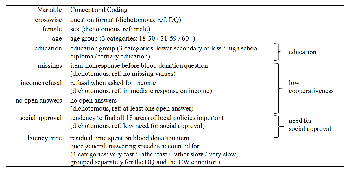
All the explanatory variables are listed in Table 4. Apart from the question format, education background and the proxies for willingness to cooperate, need for social approval and latency time, we included sex and age as control variables in our analysis (see section II in the appendix for more details on coding).

 

Table 4. Explanatory variables

 

To test our hypotheses, we used regressions adapted for randomized response data, as implemented in Stata by Jann (2005; 2008). Since we know that the prevalence of the sensitive question is , regression models can be fit by using a transformed response variable, which indicates the answer “yes” to the sensitive question for the CM condition and reduces to an ordinary dichotomous variable for the DQ condition (for details see Jann, Jerke, & Krumpal 2012: 40 et seq). This procedure allows us to analyse both experimental conditions simultaneously, meaning that we can see how the question format effect on the tendency to answer the sensitive question with “yes” changes if we add more explanatory variables to the model.

Table 5 reports the average marginal effects (AMEs) obtained from running a logistic regression to explain the tendency to answer the blood donation question with “yes”.[5] Positive effects thus indicate higher prevalence rates and, as established earlier, lower data quality in our specific case. The first model only includes the question format indicator (CM vs DQ), that is, the crucial effect of the experimental condition in which we are interested. Model 2 additionally includes all the respondent characteristics discussed before. Only the latency times are not added until Model 3. Since data on response time is only available for the online sample, the number of observations is considerably smaller in this last column. The question format effect we observe in the first (otherwise empty) model remains significant throughout the other model specifications. This means that accounting for all the discussed explanatory variables leaves the difference in response behaviour due to experimental condition unchanged.

 

Table 5. Logistic regression of tendency to answer the blood donation question positively: AMEs

To gain further insights into the mechanisms underlying the results, we estimated additional subgroup analyses to compare the estimated prevalence rates from the two experimental conditions for different respondent subgroups. Figure 2 combines data from 20 different linear regression models on sample subgroups. From each regression, only the CM coefficient (with the reference category DQ) is displayed, although we controlled for the remaining explanatory variables sex, age, education, indicators for cooperation, and need for social approval. Since latency times were only available for the online sample, the respective coefficients were calculated on the basis of a limited number of cases. All other coefficients refer to the whole sample, including online and paper questionnaires.

 

Figure 2. Crosswise coefficient for different subgroups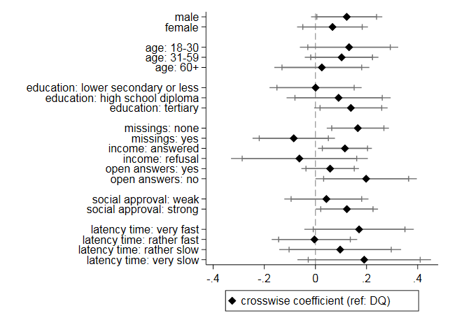

A first eye-catching result is that most coefficients are positive, meaning that the CM condition tends to yield higher estimates – and thus lower data accuracy – than the DQ condition for the vast majority of subgroups. Some of the results contradict our hypotheses. Lower educated respondents answer very similarly irrespective of experimental condition, although it was expected that this group would find the CM format particularly challenging (Hypothesis 1). Furthermore, two of three indicators for cooperation, namely the occurrence of missing values and refusals to the income question, show unexpected directions (Hypothesis 2): the respondents high in cooperativeness have higher (more unrealistic) prevalence rates in the CM than in the DQ condition, while the CM procedure worked better for uncooperative respondents. Only the absence of open answers goes hand in hand with elevated prevalence estimates in the CM, as expected. Similarly, respondents with a higher need for social approval tend to over-report blood donation in the more complex CM format, as suggested by Hypothesis 3. However, except for the interaction effect between the occurrence of missing values and experimental condition (p=0.02), none of the other interactions is statistically significant. The same is true for latency times: although we find the u-shaped pattern expected according to Hypothesis 4, groups do not differ significantly from each other. All in all, there is no support, or only weak support, for our hypotheses.

 

Discussion

This paper has been dedicated to the CM, which has been presented as an alternative to classical RRT designs and aims to reduce SDB more reliably in sensitive questions. We have presented one of the very few validation studies on the CM that exist to date. To overcome some of the key limitations prevailing in current research, we elaborated a strategy to empirically distinguish random ticking from a successful reduction of SDB in CMs. In contrast with the large majority of RRT and CM implementations, we did not assess a deviant but a socially desirable behaviour with a low prevalence rate, namely blood donation. This procedure allowed us to identify problems if respondents did not understand the question format and tended to answer randomly.

The results from our general population survey experiment on blood donation seriously limit the positive reception the CM has received in the survey research so far. A comparison with the real prevalence rate and a control group that answered a DQ format clearly shows that the CM does not help reduce SDB but, on the contrary, makes things worse. Given a heterogeneous population sample, we conclude that the CM cannot rule out factors that foster SDB but creates question-related problems, most probably because of the still high complexity inherent to the technique.

We have discussed some possible mechanisms that could explain our results (namely cognitive overburdening, unwillingness to cooperate and need for social approval), but could not find empirical evidence for any of them. Put differently, we could not identify any subgroup of respondents, in which the CM successfully reduced SDB. Only the respondents who performed their response task especially fast or slow showed a tendency to answer the CM question more inaccurately. This finding suggests an inverted u-shaped correlation between response time and data accuracy. We suspect that, particularly in the online survey, fast respondents might not fully read the instructions describing the CM format.

Following a reviewer’s comment, we would like to point out that (apart from SDB) also telescoping could in principal be part of the explanation why respondents overestimate how often they donate blood. However, it cannot explain the differences we find between the two experimental conditions. Due to randomisation, telescoping should be as likely to cause deviations from the true values in the direct question as it is in the CM condition.

One limitation of our study is that hypotheses were formulated ex post after the results of our experiment were available. Some of the concepts could have been operationalized in a more convincing way if the questionnaire had been designed for this purpose beforehand.

Moreover, we could not distinguish between over- and under-reporting, and referred only to an aggregate overall prevalence rate. Strictly speaking, our data allows judgements about the minimum number of respondents who over-reported their commitment to donate blood in the CM condition, assuming that no respondent who actually donated blood concealed this socially desirable behaviour. However, under-reporting could also exist in principle, and would implicate an even more serious problem of random tickers.

Another possibility that we unfortunately cannot test with the data at hand is that the CM triggers privacy concerns that the respondents did not have beforehand. This was suggested by at least two comments left by participants in a text box on the last page of the survey.

In sum, our evaluation study raises serious concerns about the applicability of the CM in heterogeneous population samples. Future research will have to show if there are circumstances (with regard to respondent groups, question types, survey modes and design features) under which the CM reliably reduces SDB. Until then, we would recommend other researchers to implement this question format with caution, that is, in settings that allow them to identify potential problems. One possible approach (even if validation data on the individual level is not available) has been shown here: We argued that CMs should preferably be used to elicit desirable behaviours with low prevalence rates and undesirable behaviours with high prevalence rates, in combination with a DQ condition.

Appendix

[1] This seems to be a realistic assumption. In a study where respondents were asked explicitly if they had understood the CM, 16 percent admitted that they had not, and another 21 percent stated that they had not understood the exact procedure (Kundt 2014:8). In a different study where pupils were explicitly asked for the response strategies they had applied in dealing with the CM question, 13.3 percent admitted that they had ticked answers randomly (Enzmann 2017).

[2] We want to thank Katrin Auspurg, who had this crucial idea for our experimental design.

[3] In our concrete case, asking for the last twelve months rather than lifetime prevalence allowed us to look at local blood donation events that had taken place within 2012. Unfortunately, we only had information on the number of people who donated blood for the first time as well as on the total number of donations from repeated donors, but we do not know how often the repeated donors participated. Nonetheless, the official data can at least give us a rough estimate to better evaluate the results of our survey.

[4] We also checked for mode effects, that is, for differences between online and paper questionnaires. While there was no difference in estimates for the DQ, the CM estimators differed vastly: the prevalence rate was 22 percent in the online sample, but only 4 percent in the paper questionnaires. According to the Red Cross data, this latter number is very close to the suspected true population parameter. This finding is in line with a result that Enzmann (2017) reports for a study on pupils: although the CM is believed to have particular advantages for online data collection, it seems to perform worse here than in pen and paper surveys. Furthermore, a meta-analysis by Dodou and Winter (2014) found differences in respondents‘ approval motives (measured by SD scales) between non-randomised paper and web surveys, meaning that socio-demographic groups might vary not only in their true values but also in their tendency to distort answers. In our case, bivariate analyses on sociodemographic characteristics and survey mode suggest that this finding might (at least partly) be driven by different sample compositions. We do not, however, have a sufficient number of paper questionnaires for the CM condition to run reliable multivariate analyses on the topic.

[5] We also ran linear regressions as a robustness check. In those models, the effect of the question format only reaches a significance level of slightly above 5 percent. However, as in the logistic regressions, the effect size remains equally unchanged if further explanatory variables are added.

 

 

 

References

1. Bassili, J. N., & Scott, B. S. (1996). Response Latency as a Signal to Question Problems in Survey Research. Public Opinion Quarterly 60: 390–99.
2. Becker, R. (2006). Selective Response to Questions on Delinquency. Quality and Quantity 40: 483–498.
3. Begin, G., Boivin, M., & Bellerose, J. (1979). Sensitive Data Collection Through the Random Response Technique: Some Improvements. The Journal of Psychology 101: 53–65.
4. Bockenholt, U., & van der Heijden, P. G. M. (2007). Item Randomized-Response Models for Measuring Noncompliance: Risk-Return Perceptions, Social Influences, and Self-Protective Responses. Psychometrika 72: 245–62.
5. Coutts, E., & Jann, B. (2011). Sensitive Questions in Online Surveys: Experimental Results for the Randomized Response Technique (RRT) and the Unmatched Count Technique (UCT). Sociological Methods & Research 40: 169–93.
6. Coutts, E., Jann, B., Krumpal, I., & Näher, A. (2011). Plagiarism in Student Papers: Prevalence Estimates Using Special Techniques for Sensitive Questions. Jahrbücher für Nationalökonomie und Statistik 231: 749–60.
7. Diekmann, A. (2014). Empirische Sozialforschung: Grundlagen, Methoden, Anwendungen. Rowohlt.
8. Dodou, D., & de Winter, J. C. F. (2014). Social desirability is the same in offline, online and paper surveys: A meta-analysis. Computers in Human Behavior, 36: 487-495.
9. Draisma, S., & Dijkstra, W. (2004). Response Latency and (Para)Linguistic Expressions as Indicators of Response Error. In Presser, S., Rothgeb, J. M., Couper, M. P., Lessler, J.T., Martin, E., Martin, J., & Singer, E. (eds.) Methods for Testing and Evaluating Survey Questionnaires (pp. 131–47). John Wiley & Sons.
10. Edgell, S.E., Himmelfarb, S., & Duchan, K. L. (1982). Validity of Forced Responses in a Randomized Response Model. Sociological Methods & Research 11: 89–100.
11. Enzmann, D. (2017). Die Anwendbarkeit Des Crosswise-Modells Zur Prüfung Kultureller Unterschiede Sozial Erwünschten Antwortverhaltens. In Eifler, S. & Faulbaum, F. (eds.) Methodische Probleme von Mixed-Mode-Ansätzen in der Umfrageforschung (pp. 239–77). Wiesbaden: Springer Fachmedien Wiesbaden.
12. Groves, R. M., Fowler Jr., F. J., Couper, M. P., Lepkowski, J. M., Singer, E., & Tourangeau, R. (2009). Survey Methodology. Hoboken, NJ: Wiley.
13. Himmelfarb, S. & Lickteig, C. (1982). Social Desirability and the Randomized Response Technique. Journal of Personality and Social Psychology 43: 710–17.
14. Hinz, T., Mozer, K., & Walzenbach, S. (2014). Politische Beteiligung, Konziljubiläum Und Lebenszufriedenheit. Ergebnisse der Konstanzer Bürgerbefragung 2013 – 6. Welle. Statistik Bericht 2/2014, Stadt Konstanz (http://Nbn-Resolving.de/urn:nbn:de:bsz:352-0-314600).
15. Hoffmann, A., Diedenhofen, B., Verschuere, B., & Musch, J. (2015). A Strong Validation of the Crosswise Model Using Experimentally-Induced Cheating Behavior. Experimental Psychology 62: 403–14.
16. Hoffmann, A., & Musch, J. (2016). Assessing the Validity of Two Indirect Questioning Techniques. A Stochastic Lie Detector versus the Crosswise Model. Behavior Research Methods 48: 1032–46.
17. Höglinger, M., & Diekmann, A. (2017). Uncovering a Blind Spot in Sensitive Question Research: False Positives Undermine the Crosswise-Model RRT. Political Analysis 25(1): 131–137.
18. Höglinger, M., Jann, B., & Diekmann, A. (2016). Sensitive Questions in Online Surveys: An Experimental Evaluation of Different Implementations of the Randomized Response Technique and the Crosswise Model. Survey Research Methods 10(3): 171–87.
19. Höglinger, M., Jann, B., & Diekmann, A. (2014). Sensitive Questions in Online Surveys: An Experimental Comparison of the Randomized Response Technique and the Crosswise Model. University of Bern Social Sciences Working Papers No.9. Retrieved April 21, 2015 (http://repec.sowi.unibe.ch/files/wp9/hoeglinger-jann-diekmann-2014.pdf).
20. Holbrook, A. L., & Krosnick, J. A. (2010). Measuring Voter Turnout By Using The Randomized Response Technique Evidence Calling Into Question The Method’s Validity. Public Opinion Quarterly 74: 328–43.
21. Holtgraves, T. (2004). Social Desirability and Self-Reports: Testing Models of Socially Desirable Responding. Personality & Social Psychology Bulletin 30: 161–72.
22. Jann, B. (2005). RRLOGIT: Stata Module to Estimate Logistic Regression for Randomized Response Data.
23. Jann, B. (2008). RRREG: Stata Module to Estimate Linear Probability Model for Randomized Response Data.
24. Jann, B., Jerke, J., & Krumpal, I. (2012). Asking Sensitive Questions Using the Crosswise Model An Experimental Survey Measuring Plagiarism. Public Opinion Quarterly 76: 32–49.
25. John, L. K., Loewenstein, G., Acquisti, A., & Vosgerau, J. (2013). Paradoxical Effects of Randomized Response Techniques. Working Paper. Retrieved May 4, 2016 (http://www.ofuturescholar.com/paperpage?docid=2240542).
26. Kirchner, A., Krumpal, I., Trappmann, M., & von Hermanni, H. (2013). Messung und Erklarung von Schwarzarbeit in Deutschland – Eine empirische Befragungsstudie unter besonderer Berücksichtigung des Problems der sozialen Erwünschtheit. Zeitschrift für Soziologie 42: 291–314.
27. Knowles, E. S., & Condon, C. A. (1999). Why People Say ‘yes’: A Dual-Process Theory of Acquiescence. Journal of Personality and Social Psychology 77: 379–86.
28. Korndörfer, M., Krumpal, I., & Schmukle, S. C. (2014). Measuring and Explaining Tax Evasion: Improving Self-Reports Using the Crosswise Model. Journal of Economic Psychology 45(1): 18–32.
29. Krosnick, J. A. (1991). Response Strategies for Coping with the Cognitive Demands of Attitude Measures in Surveys. Applied Cognitive Psychology 5: 213–36.
30. Krumpal, I. (2013). Determinants of social desirability bias in sensitive surveys: a literature review. Quality and Quantity 47: 2025-2047.
31. Krumpal, I. (2012). Estimating the Prevalence of Xenophobia and Anti-Semitism in Germany: A Comparison of Randomized Response and Direct Questioning. Social Science Research 41: 1387–1403.
32. Krumpal, I., & Näher, A. (2012). Entstehungsbedingungen Sozial Erwünschten Antwortverhaltens. Soziale Welt 63: 65–89.
33. Kundt, T. C. (2014). Applying ‘Benford’s Law’ to the Crosswise Model: Findings from an Online Survey on Tax Evasion. Discussion Paper. University of the German Federal Armed Forces. Retrieved May 4, 2016 (http://papers.ssrn.com/sol3/papers.cfm?abstract_id=2487069).
34. Kundt, T. C., Misch, F., & Nerre, B. (2013). Re-Assessing the Merits of Measuring Tax Evasions through Surveys: Evidence from Serbian Firms. ZEW Discussion Paper 13-047. Retrieved May 27, 2016 (http://ftp.zew.de/pub/zewdocs/dp/dp13047.pdf).
35. Landsheer, J. A., van der Heijden, P., & Van Gils, G. (1999). Trust and Understanding, Two Psychological Aspects of Randomized Response. Quality and Quantity 33: 1–12.
36. Lensvelt-Mulders, G. J. L. M. (2008). Surveying Sensitive Topics. In de Leeuw, E. D., Hox, J. J., & Dillman, D. A. (eds.) International Handbook of Survey Methodology (pp. 461–78). Lawrence Erlbaum Ass.
37. Lensvelt-Mulders, G. J. L. M., Hox, J. J., van der Heijden, P. G. M., & Maas, C. J. M. (2005). Meta-Analysis of Randomized Response Research Thirty-Five Years of Validation. Sociological Methods & Research 33: 319–48.
38. Locander, W., Sudman, S., & Bradburn, N. (1976). An Investigation of Interview Method, Threat and Response Distortion. Journal of the American Statistical Association 71(2): 269–75.
39. Mayerl, J. (2013). Response Latency Measurement in Surveys. Detecting Strong Attitudes and Response Effects. Survey Methods: Insights from the Field. Retrieved December 20, 2018 (https://surveyinsights.org/?p=1063).
40. Mayerl, J., Sellke, P., & Urban, D. (2005). Analyzing Cognitive Processes in CATI Surveys with Response Latencies: An Empirical Evaluation of the Consequences of Using Different Baseline Speed Measures. Schriftenreihe des Instituts für Sozialwissenschaften der Universität Stuttgart 2.
41. Nakhaee, M. R., Pakravan, F., & Nakhaee, N. (2013). Prevalence of Use of Anabolic Steroids by Bodybuilders Using Three Methods in a City of Iran. Addiction & Health 5: 77–82.
42. Ostapczuk, M., Moshagen, M., Zhaor, Z., & Musch, J. (2009). Assessing Sensitive Attributes Using the Randomized Response Technique: Evidence for the Importance of Response Symmetry. Journal of Educational and Behavioral Statistics 34: 267–87.
43. Ostapczuk, M., Musch, J., & Moshagen, M. (2011). Improving Self-Report Measures of Medication Non-Adherence Using a Cheating Detection Extension of the Randomized-Response Technique. Statistical Methods in Medical Research 20: 489–503.
44. Paulhus, D. (2002). Socially Desirable Responding: The Evolution of a Construct. In Braun, H., Jackson, D., & Wiley, D. (eds.) The role of constructs in psychological and educa­tional measurement. Mahwah: Erlbaum.
45. Shamsipour, M., Yunesian, M., Fotouhi, A., Jann, B., Rahimi-Movaghar, A., Asghari, F., & Akhlaghi, A. A. (2014). Estimating the Prevalence of Illicit Drug Use Among Students Using the Crosswise Model. Substance Use & Misuse 49(10): 1303-1310.
46. Stocké, V. (2007). The Interdependence of Determinants for the Strength and Direction of Social Desirability Bias in Racial Attitude Surveys. Journal of Official Statistics, 23(4): 493-514.
47. Tourangeau, R., & Yan, T. (2007). Sensitive Questions in Surveys. Psychological Bulletin 133(5): 859–883.
48. Umesh, U. N., & Peterson, R. A. (1991). A Critical Evaluation of the Randomized Response Method. Applications, Validations and Research Agenda. Sociological Methods & Research 20: 104–38.
49. Van der Heijden, P. G. M., van Gils, G., Bouts, J., & Hox, J. J. (2000). A Comparison of Randomized Response, Computer-Assisted Self-Interview, and Face-to-Face Direct Questioning. Eliciting Sensitive Information in the Context of Welfare and Unemployment Benefit. Sociological Methods & Research 28: 505–37.
50. Warner, S. L. (1965). Randomized Response: A Survey Technique for Eliminating Evasive Answer Bias. Journal of the American Statistical Association 60: 63–69.
51. Wolter, F. (2012). Heikle Fragen in Interviews. Eine Validierung der Randomized Response-Technik. Wiesbaden: Springer VS.
52. Wolter, F., & Preisendörfer, P. (2013). Asking Sensitive Questions: An Evaluation of the Randomized Response Technique vs. Direct Questioning Using Individual Validation Data. Sociological Methods & Research 42: 321–53.
53. Yan, T., & Tourangeau, R. (2008). Fast Times and Easy Questions: The Effects of Age, Experience and Question Complexity on Web Survey Response Times. Applied Cognitive Psychology 22: 51–68.
54. Yu, J., Tian, G., & Tang, M. (2008). Two New Models for Survey Sampling with Sensitive Characteristic: Design and Analysis. Metrika 67(3): 251–63.