Simultaneous Raking of Survey Weights at Multiple Levels

Special issue

---

Abstract

This paper discusses the problem of creating general purpose calibrated survey weights when the control totals data exist at different levels of aggregation, such as households and individuals. We present and compare three different methods. The first does the weighting in two stages, using only the household data, and then only the individual data. The second redefines targets at the individual level, if possible, and uses these targets to calibrate only the individual level weights. The third uses multipliers of household size to produce household level weights that simultaneously calibrate to the individual level totals. We discuss the advantages and disadvantages of these approaches, including control total data accessibility and available software from the perspective a survey statistician working outside of a national statistical organization. We conclude by outlining directions for further research.

Keywords

calibration, household, raking, weighting

Acknowledgement

The authors would like to recognize Abt SRBI for the support and encouragement.

1.    Motivation

In social, behavioral, health and other surveys, weight calibration is commonly used to correct for non-response and coverage errors (Kott, 2006, 2009, Deville & Sarndal, 1992).  Weight calibration adjusts the survey weights so that the weighted totals (means, proportions) agree with the externally known benchmarks. The latter may come from the complete frame enumeration data (population registers available in some European countries) or other large scale high quality surveys (such as the American Community Survey (ACS) in the USA).
One commonly used implementation of calibration algorithms is iterative proportional fitting, or raking (Deming & Stephan, 1940, Kolenikov, 2014). In this algorithm, the calibration margins are adjusted one at a time (i.e., effectively post-stratified), with variables repeatedly cycled until the desirable degree of convergence is achieved. In the simplest implementations, only adjustments of proportions may be feasible, and, as shown later in this paper, this may limit the survey statistician’s ability to produce accurate weights.
Many real world populations exhibit hierarchical structure that sampling statisticians can use (or simply find unavoidable). Persons in non-institutionalized populations are nested in households; patients are nested in hospitals; students are nested in classrooms which are in turn nested in schools. Calibration target data may exist at these multiple levels. This paper demonstrates how raking can be implemented to utilize these data. The running examples in the paper are households and individuals, which are often the last two stages of selection in general population surveys. The survey data that can be used for calibration may include the number of adults in the household and the household income at the household level; and age, gender, race and education at the individual level.
The problem of creating weights at different levels has been addressed in the literature in the context of household surveys in which all of the units in a household are observed. One simple approach (see e.g. Alexander, 1987) is to assign the weight of the most relevant person (e.g., the household head) to the whole household. Lemaitre & Dufour (1987) proposed a linear weighting and estimation approach that was later referred to as the generalized regression estimator (GREG) (Sarndal, Swensson, & Wretman, 2003). Lemaitre & Dufour introduced calibration variables that are defined at the individual level, and contain the household-level means of either the individual or the household variables. Alexander (1987) additionally discusses other weight calibration criteria besides least squares, including the raking ratio estimator (which he refers to as “minimum discriminant information”, MDI) and empirical likelihood estimator (which he refers to as MLE). Renssen and Nieuwenbroek (1997) extend the Lemaitre-Dufour estimator for application in the context of several surveys that share common variables. Their work is also relevant for two parts of the same survey where one part deals with households and the other with individuals. Neethling & Galpin (2006) consider weighting based on either household only or both household and individual level variables. Similar to Lemaitre & Dufour (1987), they define the variables as household averages. Neethling & Galpin (2006) also extend the class of estimators to include cosmetic estimators (Brewer, 1999) which are motivated by the combined survey inference approach (Brewer, 2002) and have improved model-based properties. Specifically, Neethling & Galpin (2006) found that using both the household and the individual level calibration improved both the accuracy and precision of the survey estimates subject to non-response.
All of these papers appear to deal with situations where all members of the household are surveyed. The weighting task is to define the household and individual weights where the individual weights within the household are equal. We are interested in a somewhat different situation where only one person per household is sampled, as is typical in most phone surveys, but additional household information can also be collected. We want to use this additional information in weight calibration.
In the demonstration, we describe and illustrate three approaches to survey weighting:

1. A two-stage process in which the household weights are produced first by calibrating only to the household targets using the base weights as input for the calibration. Then the individual weights are produced using the first stage calibrated household weights as inputs and calibrating to the individual targets only.
2. The individual weights are produced in a single pass using both the individual and household targets, but the latter are redefined at the individual level (e.g., number of individuals that live in households with exactly two adults). Here, the household weights can be produced by dividing the individual weights by the number of eligible adults in the household.
3. The household weights are produced in a single pass using the expansion multipliers (i.e., household size) from the household level to the individual level. The targets can remain at the level at which they were defined. Here, the individual weights are produced by multiplying the household weights by the expansion multipliers that were used in calibration. This approach is generally analogous to MDI-P approach of Alexander (1987; equation 5b), however, we implement it via iterative raking rather than optimization of the objective function.

These three approaches have their advantages and disadvantages. Approach 1 may be the simplest to implement, but the household weights will not benefit from the accuracy gains afforded by calibration to the individual targets. Also, the weights produced by a two-step procedure are likely to be more variable, reducing efficiency of the survey estimates (Korn & Graubard, 1999). Approaches 2 and 3 may or may not produce weights at the “other” level that are accurate for their targets. Specifically, the implied household weights from Approach 2 may or may not match the household targets, and the implied individual weights from Approach 3 may or may not match the individual targets.
The remainder of the paper compares and contrasts the three approaches outlined above. The next section introduces a numerical example based on ACS data. Then raking calibration is done using the three approaches, and the paper concludes with a short discussion of the findings. We use the Stata 12 statistical package (StataCorp. LP, 2011) for data management and analysis, and a third party raking package written by one of the authors (Kolenikov, 2014) for calibration. The complete Stata code is provided in the Appendix.
The analysis assumes a general population survey. Specialized populations can be handled by appropriate screening of the survey sampling units and subsetting the frame/population data to define the targets.

2.    Data set up

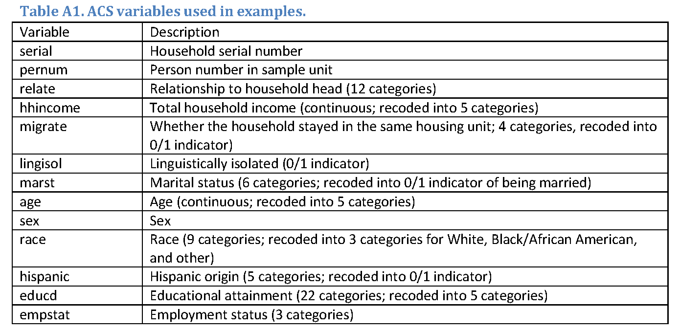
In this paper, we use one year American Community Survey (ACS) 2012 data downloaded from the IPUMS.org website (Ruggles, Alexander, Genadek, Goeken, Schroeder, & Sobek, 2010). The ACS is one of the largest continuing data collection operations in the world. Among the more than 3 million addresses  sampled each year, completed interviews are obtained from over 2 million housing units. The survey is mandatory, and achieves response rates of at least 97%. The survey asks about 50 questions on demographic and economics topics. The data are collected by web, mail, phone and in-person (in the order of modes encouraged by the Census Bureau, with the latter modes being active modes utilized for non-respondents in the web and mail modes.). The variables used in the data simulation and analysis are listed in Table 1 in Appendix 1. The full ACS dataset was subsetted to include only adults aged 18 and above, totaling 2,294,898 individuals in 1,207,415 households. The resulting (unweighted) dataset is treated as the finite population under study. The following derived variables were produced from the variables listed in Table A1:

• Defined at the household level:
  o    Household size (number of adults) with 4 categories: 1, 2, 3, 4 or more.
  o    Total household income with 5 categories: under $20,000, 20,000 to under $40,000, $40,000 to under $65,000, $65,000 to under $100,000, $100,000 and above
  o    Presence of Hispanic persons in the household: present, not present
  o    Whether the household moved within the past year: same house, moved
• Defined at the individual level for every member of the household:
  o    Race with 3 categories: White only, Black/African American only, other
  o    Education with 5 categories: below high school, high school/general education diploma, some college/associate degree, bachelor’s degree, graduate/professional degreeAge group with 5 categories: 18-29, 30-44, 45-54, 55-64 and 65 and above
  o    Marital status: married, not married

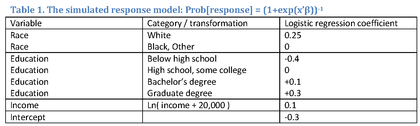
An initial simple random sample of size 5,000 households was drawn from the data, and one adult was randomly selected from each household. To produce non-trivial deviations from the population distribution of the key variables, we used logistic regression to produce a simple response model with coefficients given in Table 1. Response propensities had a mean of 0.230 and ranged from 0.129 to 0.323. In real world surveys, response propensities need to be estimated (rather than being known as in this simulation example) and usually have more variability. Individuals were considered respondents according to a Bernoulli draw with the probability of success (response) given by this model.

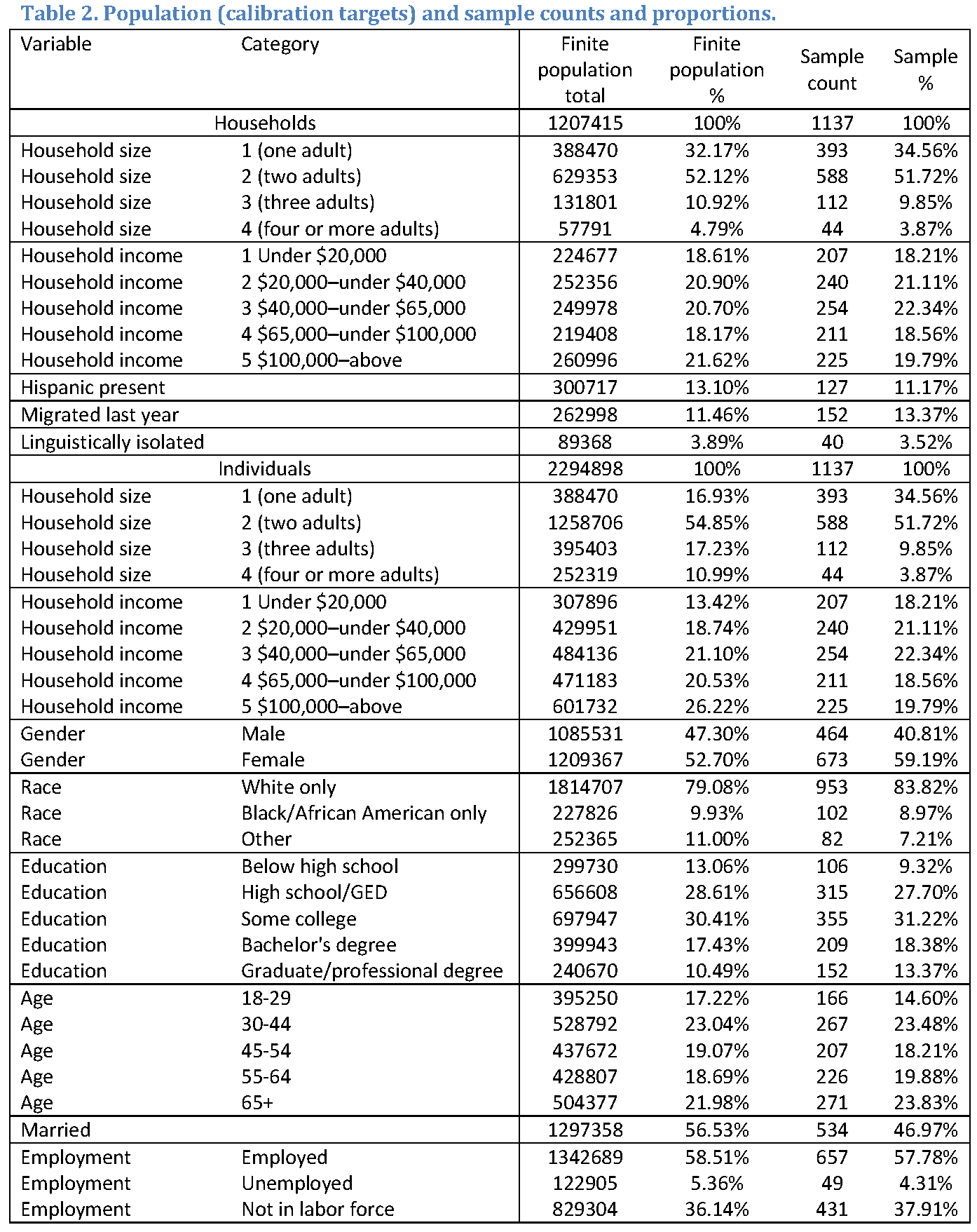
The population and sample counts and proportions are given in Table 2. The population percentages should not be considered as representative of the underlying U.S. population as the ACS weights were not used in this tabulation. The population totals listed in this table were used as raking targets.

The resulting sample has 1,137 respondents, and demonstrates some imbalances from the population proportions. This is a desirable result as it allowed the calibration methods under study to have some room to work.

 

3.    Approach 1: raking in two steps

The first approach to weighting at multiple levels is to produce weights sequentially, first for households, then for individuals. Base household weights are used as inputs for household level raking. Raked household weights multiplied by the household size are used as inputs for person level raking. Household size may be capped to avoid extreme weights, and in this example, household size was capped at 4, consistent with the categorical household size variable.
Raking converged successfully in 7 and 6 iterations, respectively. The raked weights for both households and individuals reproduce their respective targets from Table 3 within numeric accuracy (i.e., were equal to the population targets within at least six digits). Descriptive statistics for the Approach 1 weights are given in Table 5, along with those for the other approaches.

4.    Approach 2: raking individual weights using redefined targets for households

The second approach relies on redefining the population targets for households at the individual level. In other words, rather than specifying the number (or proportion) of households with income under $20,000 in the population, the targets are defined as the number of adults who live in such households. This approach requires only one raking pass that uses all the calibration variables at once. The base individual weights that combine both stages of selection (the household selection and selection of an adult within the household) can be used as input weights. Under this approach, the household weights are derived from the raked individual weights as the ratio of the raked individual weights to the household size.
Approach 2 requires access to the large scale microdata. The number of individuals residing in households of different sizes can be inferred from the household level data (if there are 10 million households with one adult, and 15 million households with two adults, we know that there are 10 million individuals residing in households with one adult, and 30 million individuals residing in households with two adults). However there is no real way to transform, for example, information on household income into the corresponding number of individuals unless the income information  is also available by household size. Households with income in the $50,000 to $75,000 range may have any number of residents, and if only the number of households in this income range is available, the number of individuals residing in them cannot be determined.
Raking converged successfully in 14 iterations. The household size was capped at 4 to avoid extremely small weights. All of the proper individual level control totals (gender, race, education, and age), as well as the household targets expressed at individual levels, were reproduced within numeric accuracy (i.e., were equal to the population targets within at least six digits), and are thus not reported. Table 3 reports the remaining household level variables. Weight summaries are reported later in Table 5 in the Discussion section. Note that Table 3 reports the results for household level variables whose convergence is not guaranteed. While household size is generally on target (as it is one of the raking margins, and for values from 1 to 3 was calibrated to the correct total) household income is not that accurate. These problematic values are shown in bold, italicized red. We consider them problematic since our expectation was that the calibration targets would have been reproduced exactly by raking.

 

5.    Approach 3: raking household weights with multipliers

The third approach rakes household level weights and uses the individual level targets via the household size multipliers. Individual level weights are then obtained as the product of household level weights and number of adults in the households (capped at 4, as in other approaches). The household base weights can be used as raking inputs only if the available raking calibration package supports raking to proportions. Otherwise, Approach 3 cannot be implemented.
In simple raking, the individual weights are proportionately adjusted so that the sum of (individual level) weights for, say, less than high school education, is equated to the number of people with this education level in the population. In the extended version of raking with multipliers, the household level weights are proportionally adjusted so that the sum of household level weights, multiplied by the household size, taken only over individuals in the sample with the specified education level, is equal to the population control total. The Stata code (Kolenikov, 2014) was designed to allow this raking modification.
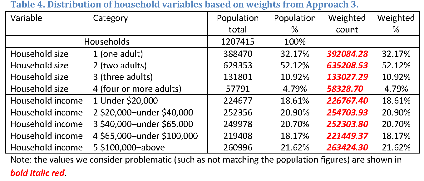
Raking converged in 15 iterations. The weighted totals for the number of adults and income (i.e., the household level variables) did not match the targets. Table 4 provides the details, with these problematic values shown in bold, italicized red. As shown in Table 4, the marginal proportions have been reproduced perfectly, meaning that the overall scale is the problem.
The scale issue is an artifact of the raking implementation in Kolenikov (2014) where the scale of the weights is determined by the last raking variable.  In this case, the last variable was age group, which is an individual level variable, and the weights inherited this variable’s scale overall. Had the last raking variable been a household level variable with control totals summing up to the number of households, we may have observed the reverse, with household targets matching both in absolute and relative terms, and individual targets being missed in absolute terms (but accurate in terms of the marginal proportions).

 

Individual level weights produced weighted distributions that matched the control totals within numeric accuracy, and are therefore not reported.

6.    Comparisons of the weights

Table 5 reports summary statistics for the raked weights with problematic values shown in bold, italicized.

 

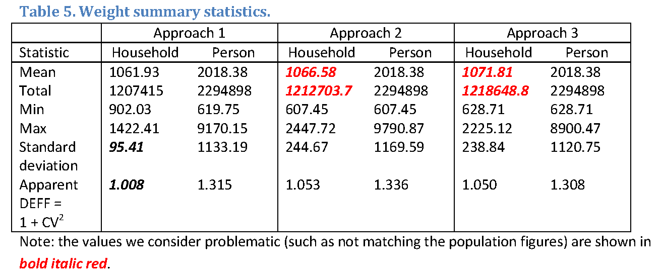
As mentioned in Section 4, household weights from Approach 2 are not sufficiently accurate for some of the household level targets. Table 5 shows that their sum does not match the population total number of households. While this problem can be easily corrected with rescaling, Section 4 also reported that the household proportions could not be matched with these weights, which is more problematic.
Although the variability of individual level weights is comparable across the three methods, the household weights from Approach 1 are less variable compared to the other two methods because they needed to satisfy fewer constraints. While less variability in the weights and lower design effects are desirable, it is hard to say whether these weights are sufficiently accurate to remove the biases in the household level variables. The next section sheds some light on the issue. Finally, the individual level weights are slightly less variable in Approach 3, but it is difficult to say whether this result is generalizable.

7.    Non-response biases

To provide an external assessment of how the different weights deal with non-response biases, we analyzed several variables from Tables 1 and 3 that were not used as calibration targets. The primary consideration is whether the 95% confidence interval based on calibrated weights covers the true population value. The confidence intervals are based on the bootstrap replicate variance estimates (Shao, 1996) implemented in Stata by (Kolenikov, 2010). Five hundred bootstrap replicates were taken, and for each replicate, all three calibrating procedures were implemented. While linearization variance estimation for Approaches 2 and 3 is feasible due to (Deville & Sarndal, 1992) who established asymptotic equivalence of calibrated estimates to GREG, it is unclear how to proceed with Approach 1. All three approaches utilize the same bootstrap frequencies in each replicate, ensuring consistent comparison of the standard errors across methods.
Table 6 reports estimates for the outcome variables, including the original population value, the estimates and confidence intervals based on the sampling weights (expanded by the overall non-response factor to produce the totals on the scale of population figures), and estimates and confidence intervals based on the calibrated weights. For each entry, the first row is the estimate; the second row is the 95% confidence interval, and in the third row, the standardized bias is the z-statistic for the null hypothesis of the true population value. As in previous tables, the problematic entries are highlighted. Table 6a reports the totals divided by 1,000, and Table 6b reports the proportions.

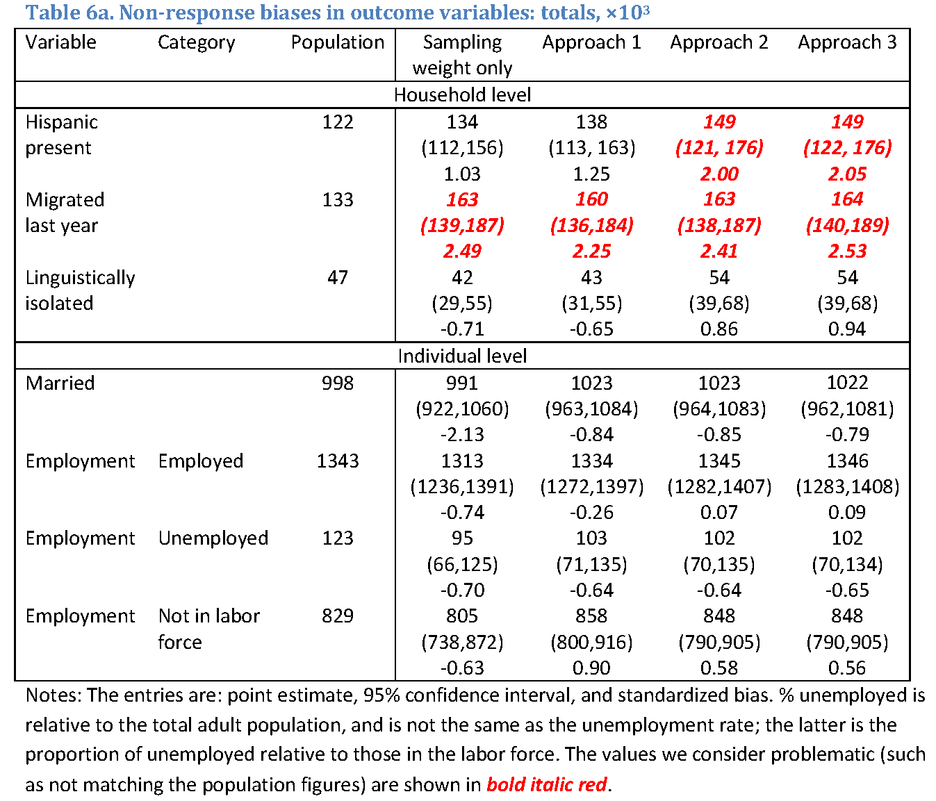
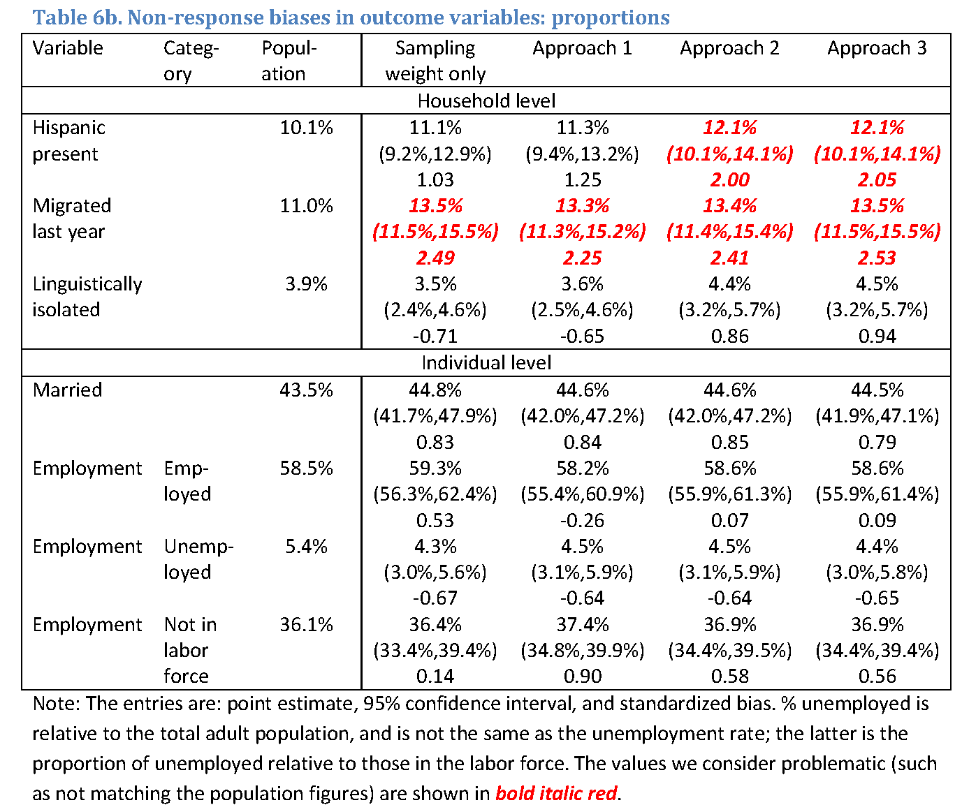
While Approaches 2 and 3 generally produce estimates that are close to one another, Approach 1 clearly produces estimates that differ from the other two approaches, as shown, for example by the linguistic isolation variable. Although the differences are not statistically significant, Approach 1 underestimates the population target by about 10% while the other two methods overestimate it by about 10%. The differences are less pronounced for the individual level variables which arguably were stronger drivers of non-response, and were subject to a greater degree of adjustment due to calibration.
None of the calibration methods successfully mitigated non-response biases in the migration variable. The responding part of the sample looked more mobile than the original population and the totals and proportions computed with calibrated weights did not move from the estimates based on the sampling weights only. Moreover, approaches 2 and 3 amplified non-response biases in the presence of Hispanic persons in the household variable, significantly overestimating it (the population target is just outside the 95% confidence interval).
Judging from the width of the confidence intervals, weight calibration produced minor efficiency gains in the employment variable, as employment is associated with education and income – both of which were used as calibration variables. For other variables, the standard errors for the estimates with calibrated weights were about the same as those based on sampling weights only. One can argue that an increase in the standard errors due to the unequal weighting effect was offset by the efficiency gains expected from calibration (Deville & Sarndal, 1992).

8.    Discussion

In this simple, controlled, simulation setting with a known response mechanism and calibration variables that were a superset of the variables determining non-response, it is reasonable to expect that perfect convergence can be achieved if one is theoretically possible. Thus any deviations from the fully accurate representation of the population figures should be seen as problematic. Approaches that do not perform well in this setting should be expected to produce greater biases in real world applications.
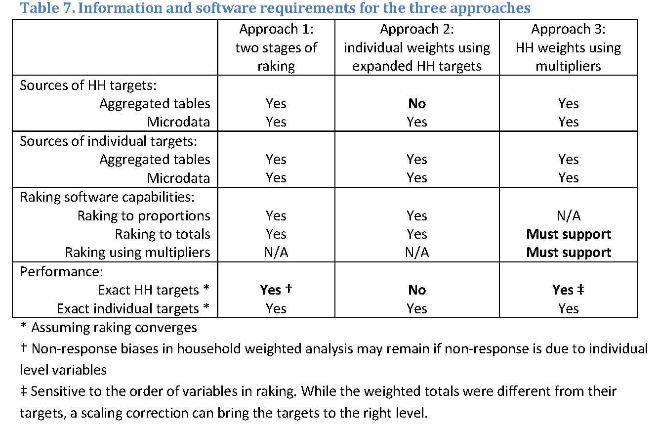
Table 7 summarizes the main features of all three approaches compared in this paper. Bold entries signify unique features of a given approach. Approach 2 requires access to microdata needed to define the targets for household level variables in terms of individual targets, and cannot be used if the aggregated data access tools provided by the national statistical offices do not produce these targets (number or proportion of people who live in households with specified characteristics).  Approach 3 is only implementable if the raking software can use population totals (rather than proportions) as controls, and if it can use multipliers (household size) rather than simply deals with sums of weights in a category to adjust raked weights.
Whereas all three methods seem to deal with individual level data without any issues, household level weights had unique quirks in each of the methods. Approach 1 does not seem to move the household weights enough, and they fail to incorporate information that is contained in the individual level variables that drive individual level weights in the other methods. Approach 2 missed some of the targets, both in absolute and relative terms. Approach 3 missed some of the targets in absolute terms, but provided accurate representation of proportions, meaning that a final pass through these weights to bring them to the right scale is called for. Both Approaches 2 and 3 produced undesirably high non-response biases in one of the household level variables. Thus, we were unable to identify the best performing approach, so in practical situations, survey statisticians can use any of them depending on the availability of calibration totals and the software.

Approach 3 was used by the current authors in calibrating the final survey weights for Wave 3 of the National Survey of Children’s Exposure to Violence (NatSCEV III) (Finkelhor, Turner, Ormrod, & Hamby, 2009). NatSCEV is the most comprehensive national survey of the incidence and prevalence of children’s exposure to violence in the U.S.  Each of the three repeated cross-sectional surveys has been conducted with computer-assisted telephone interviewing (CATI). NatSCEV III used a multiple frame design that included cell and landline RDD frames, an ABS frame, a listed landline frame, and a pre-screened probability sample of households with children. In this survey, the weights were calibrated to a mix of the household level variables (landline and cell phone use, household size, income), parent level variables (education, employment status), and child level variables (age, gender, race and ethnicity).
While this paper provides a very limited analysis of three feasible options, unanswered questions remain.  A common practice in practical weight production is weight trimming, where extremely large weights are decreased to reduce their influence, and extremely small weights are increased so that the corresponding observations contribute non-negligible amount of information to the final figures. Trimming is aimed at increasing the effective sample size by reducing weight variability. However, this reduction comes at a price of increasing biases. Overall, the effect on the mean squared error of the estimates is unclear. Moreover, the effect of trimming as a source of bias in the context of weighting at multiple levels is also unclear. This paper was only aimed at comparison of the approaches that incorporate both household and individual level variables in raking. Evaluation of trimming and its effects is outside the scope of this paper.

Appendix 1: Data

Appendix 2: Stata code

A separate online appendix provides the complete Stata code used in the above examples. It assumes that the ACS data with the necessary variables have been downloaded on the reader’s computer. ACS data in Stata format can be downloaded from IPUMS.org website at Minnesota Population Center, http://ipums.org (Ruggles, Alexander, Genadek, Goeken, Schroeder, & Sobek, 2010). The raking package by Kolenikov (2014) can be downloaded from http://www.stata-journal.com; the exact link can be found by typing “findit ipfraking” and following the instructions inside Stata. (Note that files had to be renamed into *.txt to be uploaded to the Survey Insights website; the readers are advised to rename them to *.do files traditional to Stata.)

smif-weighting-multiple-levels-prepare-data

smif-weighting-kolenikov-multiple-levels

smf-weighting-multiple-levels-results

 

References

1. Alexander, C. H. (1987). A class of methods for using person controls in household weighting. Survey Methodology, 13(1), 183-198.
2. Brewer, K. R. (1999). Cosmetic calibration with unequal probability sampling. Survey Methodology, 25(2), 205-212.
3. Brewer, K. R. (2002). Combined Survey Sampling Inference: Weighting Basu’s Elephants. London, UK: Arnold.
4. Deming, E., & Stephan, F. (1940). On a Least Squares Adjustment of a Sampled Frequency Table When the Expected Marginal Totals are Known. Annals of Mathematical Statistics, 11(4), 427-444.
5. Deville, J., & Sarndal, C. (1992). Calibration estimators in survey sampling. Journal of the American Statistical Association, 87(418), 376-382.
6. Finkelhor, D., Turner, H. A., Ormrod, R. K., & Hamby, S. L. (2009). Violence, abuse, and crime exposure in a national sample of children and youth. Pediatrics , 124(5), 1-14.
7. Kolenikov, S. (2010). Resampling variance estimation for complex survey data. The Stata Journal, 10(2), 165-199.
8. Kolenikov, S. (2014). Calibrating survey data using iterative proportional fitting (raking). The Stata Journal, 14(1), 22-59.
9. Korn, E., & Graubard, B. (1999). Analysis of Health Surveys. New York, USA: Wiley.
10. Kott, P. S. (2006). Using calibration weighting to adjust for nonresponse and coverage errors. Survey Methodology, 32(2), 133-142.
11. Kott, P. S. (2009). Calibration Weighting: Combining Probability Samples and Linear Prediction Models. In D. Pfeffermann, & C. Rao (Eds.), Handbook of Statistics: Sample Surveys: Inference and Analysis (Vol. 29B, pp. 55-82). Amsterdam, The Netherlands: Elsevier.
12. Lemaitre, G., & Dufour, J. (1987). An Integrated Method for Weighting Persons and Families. Survey Methodology, 13(2), 199-207.
13. Neethling, A., & Galpin, J. S. (2006). Weighting of Household Survey Data: A Comparison of Various Calibration, Integrated and Cosmetic Estimators. South African Statistical Journal, 40, 123-150.
14. Renssen, R. H., & Nieuwenbroek, N. J. (1997). Aligning Estimates for Common Variables in Two or More Sample Surveys. Journal of the American Statistical Association, 92(437), 368-374.
15. Ruggles, S., Alexander, J., Genadek, K., Goeken, R., Schroeder, M., & Sobek, M. (2010). Integrated Public Use Microdata Series: Version 5.0 [Machine-readable database]. Retrieved June 13, 2014, from https://usa.ipums.org/usa
16. Sarndal, C.-E., Swensson, B., & Wretman, J. (2003). Model Assisted Survey Sampling. New York, NY: Springer.
17. Shao, J. (1996). Resampling methods in sample surveys. Statistics, 27, 203-254.
18. StataCorp. LP. (2011). Stata: Release 12. Statistical Software. College Station, TX, USA.