The utility of auxiliary data for survey response modeling: Evidence from the German Internet Panel

---

Abstract

Auxiliary data are becoming more important as nonresponse rates increase and new fieldwork monitoring and respondent targeting strategies develop. In many cases, auxiliary data are collected or linked to the gross sample to predict survey response. If the auxiliary data have high predictive power, the response models can meaningfully inform survey operations as well as post-survey adjustment procedures. In this paper, I examine the utility of different sources of auxiliary data (sampling frame data, interviewer observations, and micro-geographic area data) for modeling survey response in a probability-based online panel in Germany. I find that the utility of each of these data sources is challenged by a number of concerns (scarcity, missing data, transparency issues, and high levels of aggregation) and that none of the auxiliary data are associated with survey response to any substantial degree.

Keywords

auxiliary data, INKAR data, interviewer observations, Microm data, Nonresponse, online panel recruitment, response propensity

Acknowledgement

This paper uses data from the German Internet Panel (GIP) 2012 and 2014 recruitment and registration surveys. The GIP is funded by the German Research Foundation (Deutsche Forschungsgemeinschaft, DFG) through the Collaborative Research Center (SFB) 884 "Political Economy of Reforms" (SFB 884; Project-ID 139943784). The author gratefully acknowledges the support of the SFB 884, in particular of projects A8 and Z1, and from GESIS – Leibniz Institute for the Social Sciences. In addition, the author thanks Annelies Blom for advice and feedback on early versions of this paper and Nourhan Elsayed for helping prepare the manuscript.

1. Introduction

In light of decreasing survey response rates and rising concerns about nonresponse bias and cost efficiency, auxiliary data have become popular in survey methodological research in recent years. Auxiliary data are typically external to the survey data collected and, for most operational purposes, need to be available for both respondents and nonrespondents (Sinibaldi et al., 2014). Generally, auxiliary data can be used for a number of survey operational tasks, such as eligibility screening and fieldwork monitoring, as well as post-survey nonresponse adjustments, such as weighting and imputations.

Because of the current high demand for auxiliary data, there is progress in collecting more of such data and making them available to secondary data users (e.g., in the European Social Survey (ESS, 2012) and in the Health and Retirement Study (HRS, 2014)). In addition, some official institutions and commercial vendors provide aggregated auxiliary data that can be linked to survey data.

Most approaches to using auxiliary data for nonresponse research rely on the assumption that the data are of high quality (i.e., error-free) and predictive of survey response (and, for many purposes, key survey variables; Olson, 2013). This stands in contrast to the literature on auxiliary data that indicates potential errors in the auxiliary data as well as low predictive power.

This paper contributes to the survey methodological literature on auxiliary data by exploring the utility of different sources of such data in the context of the recruitment of a probability-based online panel in Germany. First, I provide an overview of the existing literature on auxiliary data and discuss the advantages and disadvantages of the data sources that were available for my study. Then, I explore whether auxiliary variables are systematically missing by survey response, whether they are significantly associated with survey response, and what their predictive power is in survey response models.

2. Uses and usefulness of auxiliary data

Auxiliary data are used for multiple purposes, many of which involve predicting survey response. One application that has been developed in recent years is model-based representativeness measures such as R-Indicators (Schouten et al., 2009), balance indicators (Särndal, 2011), or the Fraction of Missing Information (Wagner, 2010). These representativeness measures can be reported and compared across surveys or experimental fieldwork conditions after data collection to provide data users with background information on survey data quality (Schouten et al., 2012).

In addition to measuring representativeness after data collection, auxiliary data can be used for fieldwork monitoring during data collection. The National Survey of Family Growth, for instance, has integrated auxiliary data into their fieldwork monitoring dashboard (Kirgis and Lepkowski, 2010). This allows them to detect potential problems (e.g., high numbers of locked buildings in certain areas) on a daily basis and to intervene quickly if necessary. Auxiliary data can also be used to monitor whether the sample representativeness is compromised during fieldwork, so that steps can be taken to rebalance the sample (e.g., by case-prioritization) before the fieldwork phase ends (Schouten, Shlomo, and Skinner, 2011).

A related form of auxiliary data usage occurs in responsive or adaptive survey designs (Groves and Heeringa, 2006; Wagner, 2008). The idea behind these approaches is that subgroups of the gross sample receive different survey designs depending – at least to some extent – on their response propensity as modeled using auxiliary data. Usually, the most important goal is to reduce variation in response propensities across subgroups of the gross sample. Many survey design features can be varied to reach this goal, including the survey mode or the timing of contact attempts (Schouten et al., 2013).

In a large-scale study on multiple surveys, Schouten et al. (2016) find that responsive design approaches can reduce nonresponse bias as measured by model-based representativeness measures. Similarly, Wagner et al. (2012) find that responsive design approaches based on the auxiliary data from the NSFG increase response rates among the formerly underrepresented subgroups of the sample, leading, as intended, to lower variation in response propensities across subgroups.

Another prominent application of auxiliary data is nonresponse adjustment weights (Olson, 2013), where cases are weighted by their inverse response propensity as calculated from a logistic regression model. Olson (2013) defines a useful auxiliary variable for nonresponse weighting as a variable that is associated with survey response as well as substantive survey variables of interest. This is in line with research by Little and Vartivarian (2005), who, in a simulation study, confirmed the importance of the associations between auxiliary variables and both survey response and substantive variables for creating successful nonresponse adjustments.

In an observational study on the added value of auxiliary data for the development of nonresponse adjustment weights, Kreuter et al. (2010) find that some of the available auxiliary data were useful for nonresponse adjustments while others were not. In line with Olson (2013) and Little and Vartivarian (2005), Kreuter et al. (2010) find that the auxiliary variables that were useful for nonresponse adjustments were the ones that were associated with both survey response and substantive survey variables while the auxiliary variables that were not useful showed no such associations.

3. Types of auxiliary data and their quality

Several types of auxiliary data are used in survey research and practice. The most commonly used types are sampling frame data, interviewer observations, and linked micro-geographic area data. In the following, I describe these types of auxiliary data and discuss findings from the literature about their quality.

Sampling frame data are typically available in probability-based surveys, where they describe all units in the gross survey sample. In theory, sampling frame data exist for all units on a frame. However, in practice, researchers only have access to information on the units that were actually drawn into the gross sample. Sometimes sampling frames contain a lot of information, e.g., when the sample is drawn from a register. In some countries, population registers may include detailed individual information, like age, gender, ethnic background, household composition, employment history, education history, and income. In other countries, however, the sampling frame data may be limited to broad regional information. In the literature, sampling frame data are commonly used for measuring representativeness (Schouten et al., 2009), as well as fieldwork monitoring (Schouten, Shlomo, and Skinner, 2011) and nonresponse adjustment (Kreuter et al., 2010). However, there is very little research on the quality of sampling frame data (Hall, 2008).

Interviewer observations contain information about all sample units in the gross sample. This information is recorded by interviewers during fieldwork (Olson, 2013). Commonly collected interviewer observations include reports about access impediments to the sample unit’s house (e.g., closed gates) and the type of housing unit in which the sample unit lives (e.g., single house, terraced house, apartment block, or farm; West & Kreuter, 2013). Depending on the survey, collected interviewer observations may also include interviewer assessments about the volume of traffic and public transportation stops near the housing unit (e.g., in the HRS; HRS, 2014) or interviewers’ guesses about the presence of children in a sampled household or whether the sample units are sexually active (e.g., in the NSFG; West, 2010).

Some studies evaluate the quality of interviewer observations. One finding from this research is that missing data rates can vary greatly across surveys and are often rather high. Matsuo et al. (2010), for example, find that in the ESS, the missing data rates for the interviewer observations range from 0.00% in Russia to 40.01% in Germany. Other researchers find that interviewer observations are prone to interviewer effects (see Olson, 2013). This is especially the case when the measures collected leave room for interpretation because interviewers can perceive the objects that they observe differently (Raudenbush & Sampson, 1999). West and Kreuter (2013), for example, show that in the NSFG, the accuracy of the interviewer observations about the presence of children in the household varies by interviewer experience.

The contribution of interviewer observations to nonresponse adjustments is unclear. West, Kreuter, and Trappmann (2014), for example, find that using interviewer observations in nonresponse adjustment weights hardly has any impact on substantive survey estimates. The authors suspect that this is due to the low predictive power of the interviewer observations in modeling survey response. However, Sinibaldi et al. (2014) find that interviewer observations were more successful than linked commercial micro-geographic area data in predicting primary substantive survey outcomes and were, therefore, better suited to inform nonresponse adjustment weighting.

Micro-geographic area data are linked to the survey data from external (official or commercial) sources and contain aggregated information that describe all sample units’ environments. Typical data from such sources include aggregate measures of income or purchasing power in each area, household composition in terms of socio-demographics, and the ethnic or religious composition of the neighborhood (West et al., 2015). These data can often be purchased from commercial marketing vendors, such as Microm (www.microm.de) in Germany, Experian (www.experian.co.uk) and TransUnion (www.transunion.co.uk) in the UK, and MSG (www.m-s-g.com) and Aristotle International Inc. (www.aristotle.com) in the US. Micro-geographic area data are also provided by some official institutions, such as the Federal Institute for Research on Building, Urban Affairs and Spatial Development (BBSR) in Germany, the Office for National Statistics (ONS) in the UK, and the Census Bureau in the US.

Micro-geographic area data are most commonly used in nonresponse adjustment weighting. The literature, however, shows that micro-geographic area data usually correlate little with survey response (West et al., 2015) and are, therefore, not useful in nonresponse adjustment procedures (Biemer & Peytchev, 2013). However, some studies show that the inclusion of micro-geographic area data in nonresponse adjustment weights can lead to shifts in survey estimates, especially when there is at least a moderate association with substantive survey variables (Kreuter et al., 2010).

A potential disadvantage of the commercial micro-geographic area data is that they have been found to be prone to errors. In a study on the quality of commercial marketing data, Pasek et al. (2014), find that these data were often inaccurate and systematically incomplete. The authors also point to transparency problems with commercial data: “Because these data are of considerable value to the private companies that aggregate them […] social scientists seem unlikely to gain a full picture” (p. 912). In addition, West et al. (2015) find only a weak agreement between identical variables in the data purchased from two different commercial data vendors. However, the authors conclude that buying micro-geographic area data might be a good investment for some survey operational tasks, such as eligibility screening, but less so when it comes to nonresponse weighting.

4. Data and methods

In my analyses, I explore the potential of sampling frame data, interviewer observations, and micro-geographic area data for modeling survey response across the recruitment stages of the GIP. In this section, I describe the survey data, auxiliary data, and analysis methods used in the study.

4.1 The German Internet Panel (GIP)

The GIP is a probability-based online panel of the general population with bi-monthly panel waves on multiple topics in the social sciences (Blom, Gathmann, Krieger, 2015). It is based on a three-stage stratified probability area sample, where areas in Germany are first sampled, then all addresses are listed within the sampled areas, and, finally, a sample of households is drawn from the address lists.

The GIP recruitment was conducted in two phases: a face-to-face recruitment interview and a subsequent online profile survey. All age-eligible household members in a household that participated in the recruitment interview were invited to participate in the subsequent online panel waves. Households that did not have access to the Internet or Internet-enabled devices were provided with the necessary equipment (Blom et al., 2017). A person was considered an online panel member from the moment that they filled out the first online survey, which contained questions on the participants’ personal profile, including socio-demographic characteristics and key substantive survey variables.

The GIP sampling and recruitment design have consequences for the availability of auxiliary data. For example, since the GIP samples from address lists, the sample members’ addresses can be linked to micro-geographic area data, an advantage that would be lacking if, for example, the sampling frame contained telephone numbers instead of addresses. In addition, the GIP face-to-face recruitment interviews make it possible to collect interviewer observations, which would not have been available if, for example, the survey recruitment had been done by postal mail.

The GIP recruited new panel members in 2012 and 2014. Because the samples were drawn independently of each other and the sampling and recruitment procedures were almost identical, I pool the two samples in my analyses. I conduct all analyses separately for the face-to-face recruitment interview and the online profile survey in order to investigate whether auxiliary data are associated with survey response in one, both or neither of the two recruitment steps. The pooled gross sample consists of 13,893 eligible households. 50.16% of the gross sample participated in the recruitment interview and 21.23% of the gross sample participated in the profile survey.

4.2 The auxiliary data

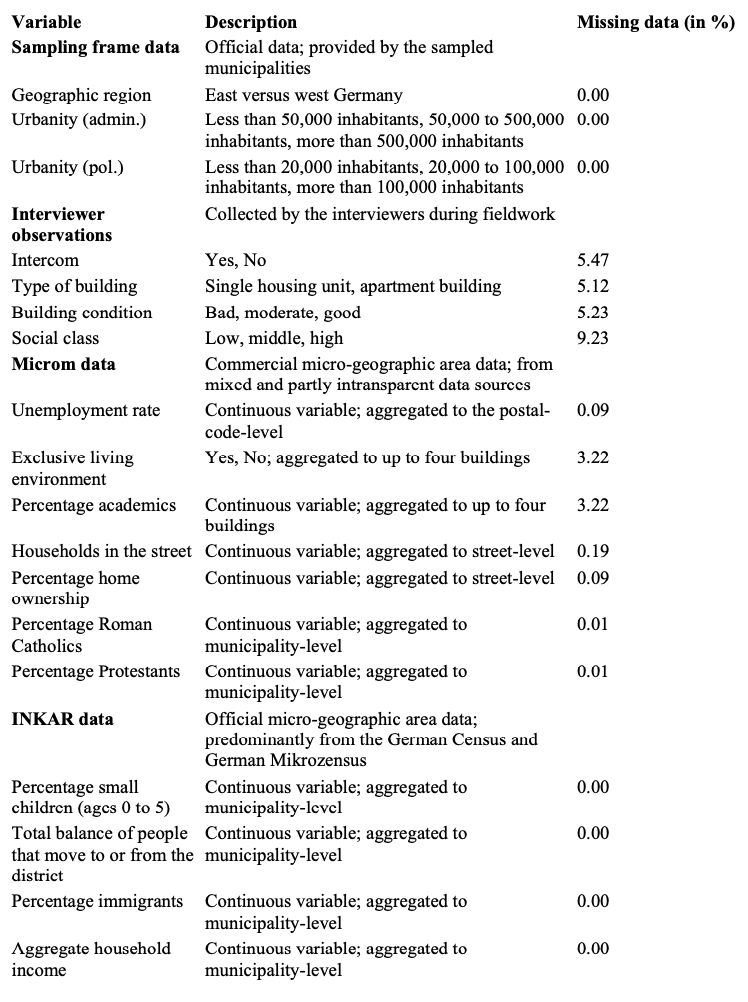
The auxiliary data used in the analyses stem from various sources. Table 1 provides an overview of the auxiliary variables, a brief description of the data, and the percentage of missing data in each variable.

Table 1: Overview of the auxiliary data, including a brief description of the data and the percentage of missing data in each variable

4.2.1 Sampling frame data

The sampling frame data in my analyses are official data from the area database from which the GIP primary sampling units are drawn. I use all the data that were available in the sampling frame. The sampling frame data include the geographic region (East versus West), the degree of urbanity operationalized as administrative districts [1] (less than 50,000 inhabitants, 50,000 to 500,000 inhabitants, more than 500,000 inhabitants), and the degree of urbanity operationalized as political governmental districts [2] (less than 20,000 inhabitants, 20,000 to 100,000 inhabitants, more than 100,000 inhabitants). The two urbanity variables measure population density in differently defined geographic areas. The sampling frame variables have no missing data.

4.2.2 Interviewer observations

The interviewers recorded fieldwork observations during the face-to-face recruitment interview. The interviewers were instructed to record observations in the contact forms for all households in the gross sample, so that the data are available for the respondents and nonrespondents. I use all the interviewer observations available from the panel recruitment process. The data include the presence of an intercom (yes, no), the type of building (single housing unit, apartment building), the building condition (bad, moderate, good), and the social class of the sampled household (low, middle, high).

These interviewer characteristics vary in the degree with which the interviewer can judge them objectively. While the presence of an intercom can usually be assessed objectively, it is unclear how interviewers can objectively determine the social class of sample units, especially in cases where the interviewer might never have seen the inhabitants of a house (i.e., for part of the nonrespondents). There is a substantial amount of missing data on all of the interviewer observations in the GIP, ranging from 5.12% on the type of building to 9.23% on social class.

4.2.3 Microm data

Microm data are micro-geographic area data provided by Microm Consumer Marketing, a commercial data vendor. The Microm data were linked to the sampled addresses of the GIP and are based on a variety of commercial and official sources, such as telecommunication providers and the German Federal Employment Agency. In the documentation of the data provided by Microm, there is little information on the data sources and aggregation procedures [3]. I use all the Microm data that were available and for which the data documentation provided, at the minimum, some hints about where the data might come from and how they might have been collected. For example, the data on the unemployment rate are reported to be provided by the German Federal Employment Agency while an “exclusive living environment” is reported to be determined by whether there are people in economic leadership positions in the neighborhood, although it is not specified how these economic leadership positions are defined and measured [3].

The variables I use in the analyses are the unemployment rate (continuous), exclusive living environment (yes, no), percentage of academics (continuous), number of households in the street (continuous), percentage of home ownership (continuous), percentage of Roman Catholics (continuous), and percentage of Protestants (continuous). Two of the variables are aggregated to up to four buildings (exclusive living environment and percentage of academics), two variables are aggregated to the street level (number of households and percentage of homeownership), two variables are aggregated to the municipality-level (percentage of Roman Catholics and percentage of Protestants), and one variable is aggregated to the postal-code-level (unemployment rate).

While it would have been desirable to include more micro-geographic area data (e.g., the percentage of Muslims in an area [i.e., not only the percentage of Roman Catholics and Protestants]), such data were not available in the dataset from the data vendor.

There is a small to moderate amount of missing data on the Microm data, ranging between 0.01% on the percentage of Roman Catholics as well as the percentage of Protestants and 3.22% on exclusive living environment as well as the percentage of academics. Unfortunately, the data vendor did not provide any documentation on why item missingness occurs in the data.

4.2.4 INKAR data

INKAR (Indicators and Maps for City and Spatial Research; Bundesinstitut für Bau-, Stadt- und Raumforschung, 2015) data are official micro-geographic area data aggregated to the municipality-level. They are predominantly based on the German Census and German Mikrozensus and can be downloaded free of charge from an Internet platform (see www.inkar.de) that is run by the German Federal Institute for Research on Building, Urban Affairs, and Spatial Development (BBSR) of the German Federal Office for Building and Regional Planning (BBR). The documentation of the data provides rich information on the data sources and adjustments. I use a selection of the INKAR data that were available on the municipality level, concerned people (rather than, for example, businesses or real estate), and that can generally be expected to be associated with survey response. The variables I used are the percentage of small children aged 0 to 5 (continuous), the total balance of people that move to or from the district (continuous), the percentage of immigrants (continuous), and the aggregate household income (continuous). Respectively, these variables operationalize the presence of small children, geographic mobility, immigration, and income, all of which have commonly been found to be associated with survey response at the individual level (e.g. Groves et al., 2011). There is no missing data on any of the INKAR data.

4.3 Methods

The analyses start with an examination of the quality of the auxiliary data in terms of item missingness. For each auxiliary variable, I examine whether there are significant differences between GIP respondents and nonrespondents regarding the proportion of missing values using Chi2-statistics.

After assessing missingness on the auxiliary data, I evaluate the utility of the different types of auxiliary data for predicting survey response: I explore the extent to which each auxiliary variable is associated with survey response using Pearson’s correlation as calculated from bivariate logistic regression models. I then estimate multivariate logistic survey response models. In these survey response models, I only include those auxiliary variables as independent variables that were statistically significantly associated with survey response in the bivariate analyses. Before including the auxiliary variables in the multivariate survey response models, I checked that there was no multicollinearity (i.e. that associations between the auxiliary variables as measured using Pearson’s correlation were all below 0.8).

To differentiate between the utility of the auxiliary variables in each panel recruitment step, I conduct separate analyses for the face-to-face recruitment interview and the subsequent online profile survey.

5. Results

5.1 Missing data

Table 2 displays, for each GIP recruitment step, the proportion of missing values among respondents and nonrespondents on each of the variables that has at least some missing values. In addition, Table 2 provides Chi2-statistics for the differences in the proportion of missing values among respondents and nonrespondents.

Table 2: Proportion of missing values and Chi2-statistics for the difference in proportion of missing values between respondents (R) and nonrespondents (NR), by auxiliary variable and GIP recruitment step (degrees of freedom (df) and p-values in parentheses; sampling frame data and INKAR data do not have any missing values)

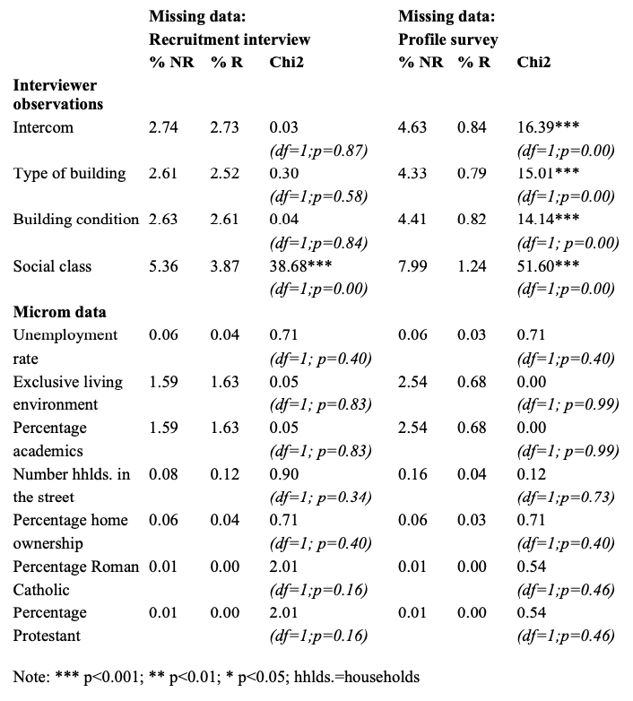
Overall, I find moderately large proportions of missing values on the interviewer observations as well as the Microm data. In the recruitment interview, the proportion of missing values is significantly higher for nonrespondents than for respondents with regard to social class. In the profile survey, the proportion of missing values is significantly higher for nonrespondents than for respondents with regard to all interviewer observations. The increase in significant differences across recruitment steps shows that sample units for which interviewer observations are missing are more likely to drop out of the panel after the recruitment interview.

5.2 Associations with survey response

Table 3 shows the association between each auxiliary variable and survey response at each GIP recruitment step.

Table 3: Association of auxiliary variables with survey response, by auxiliary variable and GIP recruitment step (Pearson’s correlation coefficients as calculated from bivariate logistic regression models)

Generally, I find that bivariate associations are small, ranging from 0.00 to 0.18. At the recruitment interview stage, no auxiliary variable is associated with survey response to any substantial degree (i.e. the correlation coefficients are smaller than 0.10). At the profile survey stage, only social class is associated with survey response, although only weakly. Despite the fact that the bivariate associations are small, a number of correlation coefficients are statistically different from 0 at a 95%-confidence level.

5.3 Predictive power in survey response models

Table 4 shows the results from the multivariate logistic regression models.

Table 4: Logistic regression models of auxiliary data on the propensity to respond in the recruitment interview and the profile survey of the GIP (models only include auxiliary variables that have been found to be significantly associated with survey response in the bivariate analyses reported in Table 3; coefficients are reported as logits, standard errors in parentheses; reference categories in parentheses)

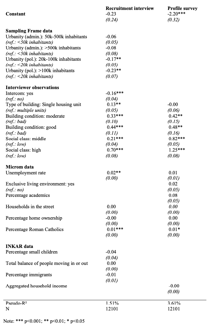
As Table 4 shows, the predictive power of the auxiliary data in the survey response models is low (Pseudo-R² of 1.51% at the recruitment interview and 3.61% at the profile survey). This is despite the fact that some of the regression coefficients are statistically significant at one or both of the recruitment stages.

6. Discussion

This study assessed the utility of auxiliary data for survey response modeling in the recruitment of the GIP, a probability-based online panel in Germany. The auxiliary data I examined were sampling frame data, interviewer observations, and commercial as well as official micro-geographic area data. Generally, I found that all of the examined auxiliary data have problems. The sampling frame data are limited to a few geographic characteristics, the interviewer observations contain relatively high proportions of missing values and the missingness is systematically related to survey response, the Microm data are insufficiently transparent, and both the Microm data and the INKAR data are aggregated to a high level. Nearly none of the auxiliary variables is substantially associated with survey response. The potential of the auxiliary data examined in this study for survey response modeling can therefore be considered to be limited.

There are a number of potential explanations for the lack of association between the auxiliary data and survey response in the GIP recruitment. One reason might be a lack in auxiliary data quality. If the data had been available on a less aggregated level and without systematically missing data, for example, they might have been able to meaningfully contribute to survey response modeling. A second explanation might be that the available auxiliary data are indeed not associated with survey response and that other types of auxiliary data would be necessary to model survey response in the GIP recruitment (e.g. voting behavior or crime rates in the neighborhood). A third potential explanation might be that the sampling and recruitment processes of the GIP are so successful in generating a balanced panel sample that there is no systematic difference between respondents and nonrespondents worth modeling. However, while the GIP is indeed successful in generating a balanced panel sample on a variety of population characteristics (e.g., age and gender), there is some evidence of systematic misrepresentation on other population characteristics (e.g., education; see Cornesse, 2018).

Overall, the results from my analyses lead to the conclusion that the currently available auxiliary data should be used with caution, because they are prone to data quality problems and might not be predictive of survey response. These problems with the auxiliary data can compromise their utility in survey operational tasks and adjustment procedures. My study shows that concerns about quality and predictive power of auxiliary data are justified and that the problems apply to a variety of commonly used types of auxiliary data. I, therefore, conclude from this research that the search for high-quality auxiliary data that is useful for survey response modeling needs to continue.

 

[1] BIK; see https://www.bik-gmbh.de/cms/basisdaten/bik-regionen for more information

[2] GKPOL; see https://www.bbsr.bund.de/BBSR/DE/Raumbeobachtung/Raumabgrenzungen/deutschland/gemeinden/StadtGemeindetyp/StadtGemeindetyp_node.html for more information

References

1. Biemer, P. P., Peytchev, A. (2013). Using Geocoded Census Data for Nonresponse Bias Correction: An Assessment. Journal of Survey Statistics and Methodology, 1(1), 24–44.
2. Blom, A. G., Gathmann, C., & Krieger, U. (2015). Setting up an online panel representative of the general population: The German Internet Panel. Field methods, 27(4), 391-408.
3. Blom, A. G., Herzing, J. M., Cornesse, C., Sakshaug, J. W., Krieger, U., & Bossert, D. (2017). Does the recruitment of offline households increase the sample representativeness of probability-based online panels? Evidence from the German internet panel. Social Science Computer Review, 0894439316651584.
4. Bundesinstitut für Bau-, Stadt- und Raumforschung (2015) INKAR: Indikatoren und Karten zur Raum- und Stadtentwicklung. © BBSR Bonn 2015. Bonn: Bundesamt für Bauwesen und Raumordnung. (Available from http://www.inkar.de.)
5. Cornesse, C. (2018). Representativeness and response quality of survey data (Doctoral dissertation). Retrieved September 20, 2019 from https://madoc.bib.uni-mannheim.de/44066/.
6. European Social Survey. (2012). ESS6 Source Contact Forms. Retrieved September 20, 2019, from the European Social Survey website: http://www.europeansocialsurvey.org/docs/round6/fieldwork/source/ESS6_source_contact_forms.pdf.
7. Groves, R. M., Fowler Jr, F. J., Couper, M. P., Lepkowski, J. M., Singer, E., & Tourangeau, R. (2011). Survey methodology (Vol. 561). John Wiley & Sons.
8. Groves, R. M., & Heeringa, S. G. (2006). Responsive design for household surveys: tools for actively controlling survey errors and costs. Journal of the Royal Statistical Society: Series A (Statistics in Society), 169(3), 439-457.
9. Hall, J. (2008). Sampling Frame. In: Paul Lavrakas (ed.) Encyclopedia of Survey Research Methods. 790-791.
10. HRS. (2014). HRS 2014 Final Release Codebook. Retrieved September 20, 2019, from the HRS website: http://hrsonline.isr.umich.edu/modules/meta/2014/core/codebook/h14_00.html.
11. Kirgis, N., & Lepkowski, J. (2010). A management model for continuous data collection: Reflections from the National Survey of Family Growth, 2006–2010. NSFG Paper, (10-011). Retrieved September 20, 2019, from the Population Studies Center website: http://citeseerx.ist.psu.edu/viewdoc/download?doi=10.1.1.642.2725&rep=rep1&type=pdf.
12. Kreuter, F., Olson, K., Wagner, J., Yan, T., Ezzati‐Rice, T. M., Casas‐Cordero, C., Lemay, M., Peytchev A., Groves, R.M., & Raghunathan, T. E. (2010). Using proxy measures and other correlates of survey outcomes to adjust for non‐response: examples from multiple surveys. Journal of the Royal Statistical Society: Series A (Statistics in Society), 173(2), 389-407.
13. Little, R. J. A. and S. Vartivarian (2005). “Does Weighting for Nonresponse Increase the Variance of Survey Means?” Survey Methodology 31(2): 161-168.
14. Matsuo, H., Billiet, J., & Loosveldt, G. (2010). Response-based quality assessment of ESS Round 4: Results for 24 countries based on contact files. Retrieved September 20, 2019, from the European Social Survey website: https://www.europeansocialsurvey.org/docs/round4/methods/ESS4_response_based_quality_assessment_e02.pdf.
15. Olson, K. (2013). Paradata for nonresponse adjustment. The ANNALS of the American Academy of Political and Social Science, 645(1), 142-170.
16. Pasek, J., Jang, S. M., Cobb III, C. L., Dennis, J. M., & Disogra, C. (2014). Can marketing data aid survey research? Examining accuracy and completeness in Consumer-File data. Public Opinion Quarterly, 78(4), 889-916.
17. Sampson, R. J., & Raudenbush, S. W. (1999). Systematic social observation of public spaces: A new look at disorder in urban neighborhoods. American journal of sociology, 105(3), 603-651.
18. Särndal, C. E. (2011). The 2010 Morris Hansen Lecture. Dealing with survey nonresponse in data collection, in estimation. Journal of Official Statistics, 27(1), 1.
19. Sakshaug, J., Antoni, M., & Sauckel, R. (2017). The Quality and Selectivity of Linking Federal Administrative Records to Respondents and Nonrespondents in a General Population Sample Survey of Germany. Survey Research Methods 11(1), 63-80.
20. Schouten, B., Cobben, F., & Bethlehem, J. (2009). Indicators for the representativeness of survey response. Survey Methodology, 35(1), 101-113.
21. Schouten, B., Calinescu, M., & Luiten, A. (2013). Optimizing quality of response through adaptive survey designs. Survey Methodology, 39(1), 29-58.
22. Schouten, B., Shlomo, N. and Skinner, C. (2011) Indicators for Monitoring and Improving Representativeness of Response. Journal of Official Statistics, 27(2), 1-24.
23. Schouten, B., Bethlehem, J., Beullens, K., Kleven, Ø., Loosveldt, G., Luiten, A., Rutar, K., Shlomo, N., & Skinner, C. (2012). Evaluating, Comparing, Monitoring, and Improving Representativeness of Survey Response Through R‐Indicators and Partial R‐Indicators. International Statistical Review, 80(3), 382-399.
24. Schouten, B., Cobben, F., Lundquist, P. and Wagner, J. (2016). Does more balanced survey response imply less non-response bias? Journal of the Royal Statistical Society, A, 179, 727–748.
25. Sinibaldi, J., Trappmann, M., & Kreuter, F. (2014). Which is the better investment for nonresponse adjustment: Purchasing commercial auxiliary data or collecting interviewer observations? Public Opinion Quarterly, 78(2), 440-473.
26. Wagner, J. R. (2008). Adaptive survey design to reduce nonresponse bias (Doctoral dissertation, University of Michigan). Retrieved September 20, 2019, from ProQuest: https://search.proquest.com/docview/304573555?pq-origsite=gscholar.
27. Wagner, J. (2010). The fraction of missing information as a tool for monitoring the quality of survey data. Public Opinion Quarterly, 74(2), 223-243.
28. Wagner, J., West, B. T., Kirgis, N., Lepkowski, J. M., Axinn, W. G., & Ndiaye, S. K. (2012). Use of paradata in a responsive design framework to manage a field data collection. Journal of Official Statistics, 28(4), 477.
29. West, B. (2010). An Examination of the Quality and Utility of Interviewer Estimates of Household Characteristics in the National Survey of Family Growth. NSFG Working Paper, (10-009). Retrieved December 6, 2017, from the Population Studies Center website: https://pdfs.semanticscholar.org/d593/09e8e9d0109c56611715e53a597bb4f1236e.pdf.
30. West, B. T., Kreuter, F., & Trappmann, M. (2014). Is the collection of interviewer observations worthwhile in an Economic Panel Survey? New evidence from the German Labor Market and Social Security (PASS) study. Journal of Survey Statistics and Methodology, 2(2), 159-181.
31. West, B. T., & Kreuter, F. (2013). Factors affecting the accuracy of interviewer observations: Evidence from the National Survey of Family Growth. Public Opinion Quarterly, 77(2), 522-548.
32. West, B. T., & Little, R. J. (2013). Non‐response adjustment of survey estimates based on auxiliary variables subject to error. Journal of the Royal Statistical Society: Series C (Applied Statistics), 62(2), 213-231.
33. West, B. T., Wagner, J., Hubbard, F., & Gu, H. (2015). The utility of alternative commercial data sources for survey operations and estimation: Evidence from the National Survey of Family Growth. Journal of Survey Statistics and Methodology, 3(2), 240-264.