Measurement Invariance and Maximal Reliability: Exploring a Potential Link

---

Abstract

A procedure for examining group differences in predictability of latent constructs with social measurement instruments is outlined. The method is developed within the framework of latent variable modeling and is widely applicable with popular software. The approach is based on the notions of maximal reliability and optimal linear combination that have been receiving increased attention over the past several decades. The procedure is readily employed for point and interval estimation of the population discrepancy in construct predictability using the instrument components. The discussed method is related to the study of measurement invariance and is illustrated with numerical data.

Keywords

construct, construct predictability, maximal reliability, measurement invariance, multi-group study, multiple-component measuring instrument, optimal linear combination

Acknowledgement

This research was supported by the Institute of Sociology of the Dresden University of Technology. We are indebted to two anonymous Referees and B. Zhang for their valuable and critical comments on an earlier version of the paper that have contributed considerably to its improvement.

Introduction

The majority of theoretical concepts of relevance in the social sciences are typically not directly observable entities, and for this reason are frequently referred to as latent constructs, traits, continua, dimensions, or factors (e.g., McDonald, 1999). These constructs – such as attitudes or abilities, for example – are only indirectly measurable, which is achieved using multiple indicators representing their presumed manifestations (e.g., Bollen, 1989). In this way, the complex nature of various latent constructs of interest can be managed and they become available for research (e.g., Mulaik, 2009). Empirical studies concerned with these unobservable variables and their interrelationships frequently utilize latent variable models that reflect sets of hypothetical relationships among the constructs as well as between them and their indicators (e.g., Raykov & Marcoulides, 2011).

A large part of such applications of latent variable modeling (LVM; Muthén, 2002) aim at facilitating inferences about constructs of empirical and theoretical concern, which are based on their observed manifestations and may be construed as seeking predictions about the latent traits using information contained in their used indicators. Trustworthy inferences about these constructs require high degree of predictability, i.e., low prediction error, which may well depend on the population under investigation. This necessitates the use of LVM that makes it possible to estimate construct predictability and its comparison across groups of interest.

The present article addresses this need by discussing a procedure for evaluating population differences in predictability of studied latent constructs using social measurement instruments in multi-population settings. The approach is based on the notions of maximal reliability (MR) and optimal linear combination (OLC), and can be used for point and interval estimation of this discrepancy in construct predictability based on the instrument components. We discuss also the potential link of these notions and approach to measurement invariance (MI), and illustrate the outlined method with numerical data.

Background, Notation, and Assumptions

In this paper, we assume that a set of k given observed variables constitute a multi-component measuring instrument under consideration (e.g., scale, self-report, survey, questionnaire, or inventory), and will denote its components by y = (y₁, y₂, …, y_k)′ (k ≥ 3; priming is used to symbolize transposition and underlining a vector in the sequel). The following discussion can be extended readily to the case of more than one studied construct, but for developing its underlying idea it suffices to assume that the instrument is unidimensional and its component errors as uncorrelated (see also discussion and conclusion section). We posit that the scale consisting of the measures in y is administered to independent samples from two or more distinct populations (referred to also as ‘groups’). For simplicity we assume that two populations are examined, but the developments below are readily generalized to the case with more than two groups. These populations are presumed not to be affected by clustering effects or substantial unobserved heterogeneity (Rabe-Hesketh & Skrondal, 2022; Geiser, 2013). The scale components or measures y₁, y₂, …, y_k are further assumed to fulfill the widely adopted configural invariance condition (e.g., Millsap, 2011). Accordingly, the following factor analysis model is stipulated in the gth group (g = 1, 2):

 

(1)                                                                 y_g = a_g + B_g f_g + e_g ,

 

where y_g denotes the k x 1 vector of the instrument components in the gth group and f_g is the underlying construct (factor) there. In addition, in Equations (1) B_g = (b_1g, …, b_kg)′ is the k x 1 vector of factor loadings in that population that are assumed positive (possibly after recoding), and a_g is the k x 1 vector of intercepts; similarly, e_g is the k x 1 vector of zero-mean residuals, presumed with positive variances and uncorrelated among themselves as well as with f_g (e.g., Mulaik, 2009; g = 1, 2). Lastly, we assume that model (1) underlying this article is identified through appropriate parameter restrictions (including zero latent mean and unit latent variance in one group, which are free parameters in the other group; e.g., Muthén & Muthén, 2025).

In the remainder of this paper, to accomplish its aims a measuring instrument (frequently referred to as scale in the sequel) is referred to as measurement invariant, if the intercepts and loadings in Equation (1) are identical across the studied groups (cf. Millsap, 2011), i.e., if the equalities a₁ = a₂ and B₁ = B₂ hold. The last two equations can be interpreted as requiring group-identity in the origins and units of measurement of the construct in question, respectively, as achieved by the instrument components. The following discussion is also concerned with exploring a potential link between the concepts of MI and MR, and exemplifies the possibility of reaching veridical conclusions about latent group mean and variance differences under certain conditions with limited violation of MI.

Maximal Reliability and the Optimal Linear Combination

The notion of MR is almost a century old (e.g., Thompson, 1940). However, during this time it has not acquired the popularity among empirically working social scientists that would be comparable to that of the commonly used scale reliability coefficient, denoted r_Y, where Y = y₁ + … + y_k is the scale component sum (often called scale score). In difference to r_Y, the MR concept pertains to that of their linear combinations Z = w₁y₁ + … + w_ky_k, referred to as optimal linear combination (OLC), which is associated with the highest reliability achievable with a linear combination of these measures y₁, …, y_k (e.g., Conger, 1980). As shown in the literature, for the single-group version of model (1), the optimal weights rendering that OLC and highest reliability associated with the latter are

 

(2)                                                                 w_j = b_j / θ_j

 

where θ_j = Var(e_j) denotes the variance of the jth component residual e_j (j = 1, …, k; e.g., Bartholomew, 1996). The MR coefficient for a scale under consideration, designated ρ, is then the reliability coefficient of the above OLC, Z, which uses the weights in Equation (2).

In a given population, the MR coefficient has been shown to equal the following function of the parameters of model (1):

 

(3)

 

(e.g., Conger, 1980). From the right-hand side of Equation (3), it is seen that MR is (i) an increasing function of the absolute value of any factor loading, all else kept constant, as well as (ii) a decreasing function of any residual variance then. In addition, the MR coefficient is (iii) an increasing function of any of the ratios

 

(4)                                                                 r_j = b_j²/θ_j

 

(j = 1, …, k), everything else held constant. We will make use of all these observations in the following sections¹.

Maximal Reliability and Predictability of a Latent Construct

Since the well-known reliability coefficient is the R-squared index of the pertinent observed measure (manifest variable) if conceptually regressed upon its true (latent) score, or conversely (e.g., McDonald, 1999), the MR coefficient can be viewed as the maximal possible R-squared index obtainable between a linear combination of the components of a given scale and the construct (factor) that it is evaluating. Therefore, finding the OLC amounts to finding those weights w₁, …, w_k, with which Z = w₁ y₁ + … + w_k y_k is maximally correlated with its underlying trait or factor score, denoted f_Z (cf. Hancock & Mueller, 2001; see also Appendix 2). Equivalently, this is the search for such component weights, with which the highest percentage of variance is explained in the latent variable f in Equation (1) (for a given group), when using an appropriate linear combination of y₁, …, y_k. In other words, with those optimal weights w₁, …, w_k the instrument components (as a set of measures) are most predictive of the studied trait. This degree of construct predictability is reflected then in the R-square index of the conceptual regression of f on the observed scale components y₁, …, y_k (see Appendix 2 for further detail and qualification). In such a regression activity, as is well known, what is sought is the linear combination of the components that possesses the highest squared correlation with the response variable (e.g., Agresti, 2018), which here is the factor f. As indicated earlier, however, this squared correlation is the MR coefficient. Hence, MR represents the maximal possible degree of (conceptual) predictability of the latent construct f, which is achievable using a linear combination of its manifestations, indicators, or proxies y₁, …, y_k (cf. Raykov et al., 2015). We utilize these relationships next.

Studying Group Differences in Construct Predictability

With the above MR interpretation in mind, an empirically important question that can next be addressed is that about the extent to which a studied latent construct’s predictability, based on a used measuring instrument, differs across examined populations. Hence, as a possible index of group differences in construct predictability (GDCP), one could view the discrepancy in the MR coefficients across two populations under consideration (cf. Raykov & Hancock, 2005). Therefore, as a measure of GDCP one can use the quantity

 

(5)                                                              Δ = |ρ₁ – ρ₂|

 

where ρ₁ denotes the MR coefficient in group 1, ρ₂ that coefficient in group 2, and |.| symbolizes absolute value. ^2,3. Appendix 2 outlines how this measure can be point and interval estimated in a social science study using the popular LVM methodology and pertinent software.

From Equation (5), it is seen that the GDCP index Δ represents the extent to which the latent construct evaluated by the used instrument would be more predictable in one of the groups than in the other group. Thereby,  Δ= 0 is a necessary and sufficient condition for the construct to be equally predictable in both populations of concern. Based on Equations (3) and (5), it is now readily realized that the GDCP is a function of all factor loadings and error variances for model (1) in each of the groups. That is, in terms of formal notation,

 

(6)                               Δ = Δ(b₁₁, …, b_k1, θ₁₁, …, θ_k1; b₁₂, …, b_k2, θ₁₂, …, θ_k2)

 

holds, where the second subindex designates population. We also notice that due to obvious group symmetry considerations, the sign of the GDCP is in general not important, but only its magnitude is of relevance. Last but not least, from its definition in Equation (5) it is seen that the GDCP index Δ does not depend on the scale component intercepts and their cross-group relations.

We further observe from Equations (3) and (5) that Δ = 0 if there is equality in all factor loadings and residual/error variances across groups. However, if some factor loadings are not group invariant, it is still possible that there is no population difference in the MR coefficients and thus Δ = 0 holds. Hence, lack of group invariance with respect to factor loadings may still go together with population equality in construct predictability based on the scale components. Thus, the concept of group difference in construct predictability is more general than that of (strict) MI, and the GDCP measure (5) can thus be an indicator of population differences in latent trait predictability also when a given instrument does not possess the property of MI. Along this line of reasoning, when (a) Δ is close to 0, (b) construct predictability is high in both groups, (c) the intercepts are group invariant, and (d) the same trait or construct is being evaluated in them on the same underlying measurement scale, then the following conjecture could be advanced. Accordingly, it may be possible that trustworthy conclusions could then be made with respect to population differences in construct means and/or variances, in case population invariance does not hold for all factor loadings. In that case, the conjecture suggests the possibility of evaluating in a potentially dependable way latent population differences. In actual fact, next we show on numerical data within an empirically relevant setting that this conjecture can be true.

Illustration on Data

In order to demonstrate the utility and applicability of the outlined GDCP evaluation procedure, as well as the possible link between MR and trustworthy conclusions about latent group differences, we utilize data simulated for a measuring instrument with k = 6 components in g = 2 groups having n₁ = n₂ = 800 cases each, with s = 10,000 replications (generated data sets). These data sets were simulated according to the model defined in the following Equations (7) (see first Mplus command file in Appendix 1, to be used along with the second Mplus command file there if willing to replicate all results in this section). Specifically, in Group 1 the following model was used (cf. Equations (1)):

 

(7)                                                              y₁ = f + e₁ ,

                                                                  y₂ = 1.5 f + e₂ , and

                                                                  y_j = 2 f + e_j

 

for j = 3, 4, 5 and 6, where e₁ through e₆ were independent zero-mean normal variates with variance 2, and f was a standard normal variate independent of them. In Group 2, the same model was used for data generation purposes, except that (i) the loading of the last component, y₆, was set at b₆₂ = 1 rather than at 2 as in Group 1; (ii) its error variance was set at θ₆₂ = .5 in lieu of θ₆₁ = 2 in Group 1; and (iii) the latent mean and variance were set at ν₂ = 0.33 and ω₂ = 1.33, respectively, in Group 2, unlike these mean and variance parameters being fixed in Group 1 correspondingly to 0 and 1 (see Equations (1); Muthén & Muthén, 2002, 2025). That is, apart from the last loading on f₁ and its error variance, both groups were invariant in all loadings, intercepts, and residual variances. In addition, relative to Group 1, the latent mean and variance were higher in Group 2 by a third of the latent variance in Group 1.

With these population parameters in mind, we note that (a) the contribution of each individual scale component to the MR coefficient, viz. its associated r-ratio (4), is the same in each group (population). Indeed, as found from Equations (4), in either group the population r-ratios for the instrument components y₁, …, y₆ are .5, 1.125, 2, 2, 2 and 2, respectively. Hence, (b) the MR coefficient (3) is invariant at the population level, i.e., ρ₁ = ρ₂ holds, and we denote this common coefficient as r next. In addition, using Equation (3), this MR ρ is found in each group to be (e.g., Bartholomew, 1996; asterisk denoting multiplication next)

 

(8)                              ρ = (1/2 + 1.5²/2 + 4_*4/2)/(1 + 1/2 + 1.5²/2 + 4_*4/2) = .906 ,

 

indicating a high level of construct predictability in each group. Furthermore, the population GDCP index (5) vanishes, i.e., Δ = 0 is true, and both groups are associated with the same construct predictability power, i.e., the underlying construct f is equally well predictable with its indicators y₁ through y₆.

We emphasize that the population latent mean and variance group differences are not zero but positive (in absolute value) here, since either of them equals a third of the latent standard deviation in Group 1. Hence, due to the equal and high level of predictability of the latent trait in both groups, according to the earlier stated conjecture one may suspect that model (1) may sense these group differences in latent mean and latent variance that were built in the data simulation process.

We therefore fit next to each of the 10,000 replications data sets the two-group model (1) with group-invariant loadings and intercepts, except the loading of the last component y₆ (as well as the latent mean and variance being fixed at 0 and 1 in Group 1 but free in Group 2). As indicated earlier, this is accomplished with the second Mplus command file in Appendix 1 (referred to as Code 2 there). As expected, the resulting goodness of fit indices indicate a tenable model, over the 10,000 replications, due to them being as follows: mean chi-square (ave – χ²) = 27.114, standard deviation (SD) = 7.458, degrees of freedom (df) = 27, and average root mean square error of approximation (ave-RMSEA) = .007 with SD = .009 (note that the .05 cut-off for the chi-square distribution with df = 27 is χ²_.05,27 = 40.113). This model plausibility conclusion is further supported by an examination of the behavior of its chi-square goodness of fit and RMSEA values across these replications, which are summarized in Table 1 and presented in histogram form in Figure 1. The relevant parameter estimates and related statistics are displayed in Table 2 (presented further below).

 

Table 1: Chi-square goodness of fit and RMSEA results across the 10,000 replications in the illustration section example (used software format).

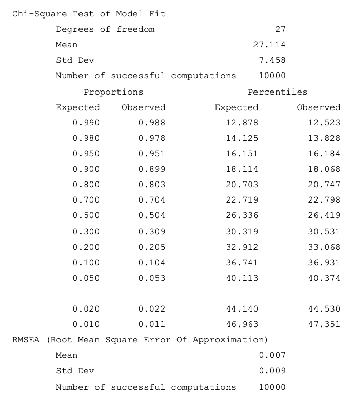
Note. See main text for specific discussion of entries of this Table and Muthén & Muthén (2025, ch. 12).

 

In the upper part of Table 1 (see its left pair of proportion columns), we notice that the empirical and theoretical reference chi-square distributions are nearly identical, which is consistent with a tenable model (e.g., Muthén & Muthén, 2025). In particular, as expected under the model, effectively 5% of the replications (more precisely, 5.3% of them) are associated with model rejection and 95% of them with a retainable model. Moreover, from the lower part of Table 1 it is seen that essentially all replications were associated with an RMSEA no higher than .05, which is an additional piece of evidence for tenable model fit (Browne & Cudeck, 1993; see also Figure 1).

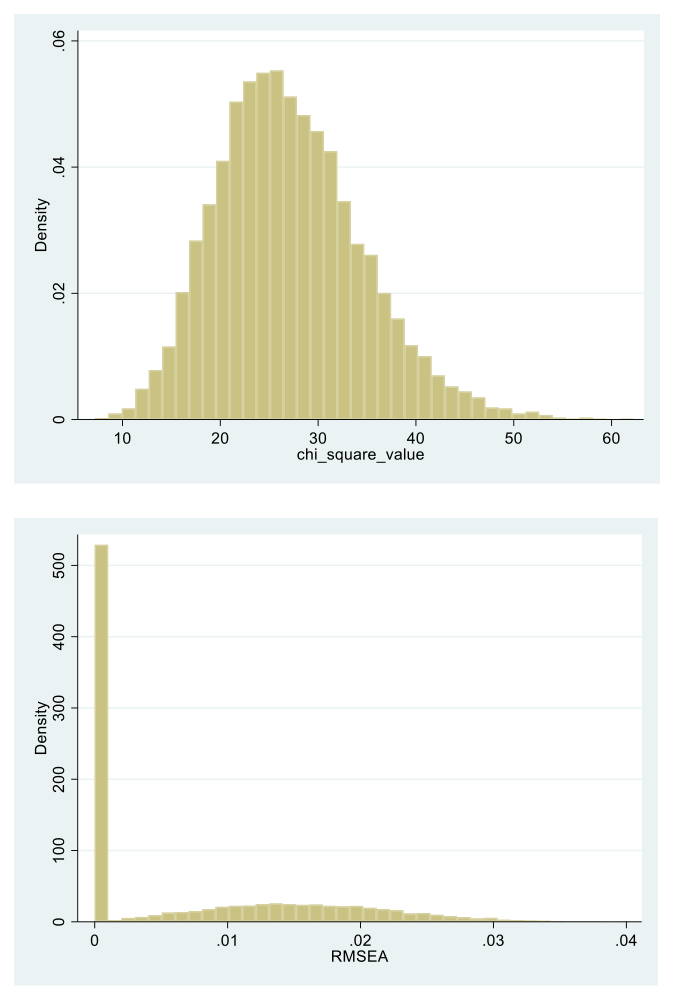
Figure 1. Histograms of the chi-square goodness of fit and root mean square error of approximation values (RMSEAs; top to bottom) for the fitted two-group, single-factor model to the 10,000 replication data sets (see Equations (1) and (7)).

 

The results in Table 1 and Figure 1 corroborate the interpretation of the fitted two-group, single-factor model as a plausible means of data description and explanation across the 10,000 replication sets. We thus proceed now to the interpretation of the model parameters of main concern. To this end, we examine the estimates of the GDCP index (5) that are summarized in the lower part of Table 2 and similarly presented graphically in Figure 2.

 

Table 2: Parameter estimate results for the single-factor model fitted to the 10,000 simulated replication data sets (see main text for details; software format used)

Note. ^a = parameter value is fixed by model definition (for identification purposes; e.g., Raykov et al., 2015), MR1 = maximal reliability coefficient in group 1, MR2 = maximal reliability coefficient in group 2, LV_G2 = latent variance in group 2; SD = standard deviation, Ave. = average, S.E. = standard error, MSE = mean squared error. (See also second Mplus command file in Appendix 2, as well as Muthén & Muthén, 2025, ch. 12, for additional explanation of entries and definitions.)

 

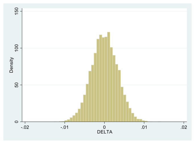
Figure 2. Histogram of the GDCP index D (named “DELTA” in Table 2 and the second Mplus command file in Appendix 1) across the 10,000 replication data sets (see Equation (5)).

 

Accordingly, across the 10,000 replications the mean GDCP estimates is  Δ^* = 0.000, with SD = .003 (see the “DELTA” row of Table 2). Furthermore, in 4.9% of the 10,000 replications the null hypothesis H₀: Δ = 0 is rejected, which percentage (effectively 5%) is expected due to chance alone (see last entry in that “DELTA” row). Relatedly, from the same part of Table 2 we see the mean of the MR estimates in each group being ρ₁^* = ρ₂^* = .906, i.e., identical to their population value (rounded-off), with SD = .005 (see Equation (8) and the two rows in Table 2 above that for “DELTA”). These estimates are graphically displayed in Figure 3 that demonstrates their nearly identical group distributions, each tightly clustered around their last stated mean, similarly to the replication distribution of the GDCP estimates.

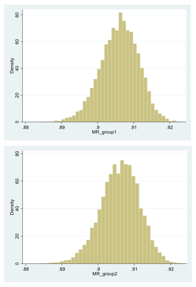
Figure 3. Histograms of the maximal reliability coefficients in Group 1 and Group 2 (top to bottom) across the 10,000 replication data sets (see Equation (3)).

The Group 2 latent mean and variance estimate distributions across the 10,000 replications are next of interest (see central part of Table 2, viz. its “Means” row in the “Group G2” output part, and Figure 4). Thereby, the mean of the latent mean estimates in that group is ν^* = .334, i.e., essentially identical to its population value, with SD = .057. Also, none of the 10,000 replication 95%-confidence intervals for this latent mean includes the point 0, and for all replications the null hypothesis of it being 0 is rejected (see last two entries in that parameter row of Table 2). These results indicate that in all replication data sets the fitted model correctly sensed the latent group mean difference. Similarly, the mean of the latent variance estimate distribution in Group 2 is found to be ω^* = 1.339, which is essentially the same as its population value, with SD = .106 (see lower part of Table 2, viz. the “Variance” row in the G2 output section). Thereby, in 93.3% of the replications the model correctly sensed the latent standard deviation difference built into the data generation process, by rejecting the null hypothesis of it being equal to 1 in the population (see last entry in last row of Table 2; note that this percentage is rather close to the nominal 95%). Further, Figure 4 presents the histograms of these latent mean and variance estimates, which highlights the reported findings.

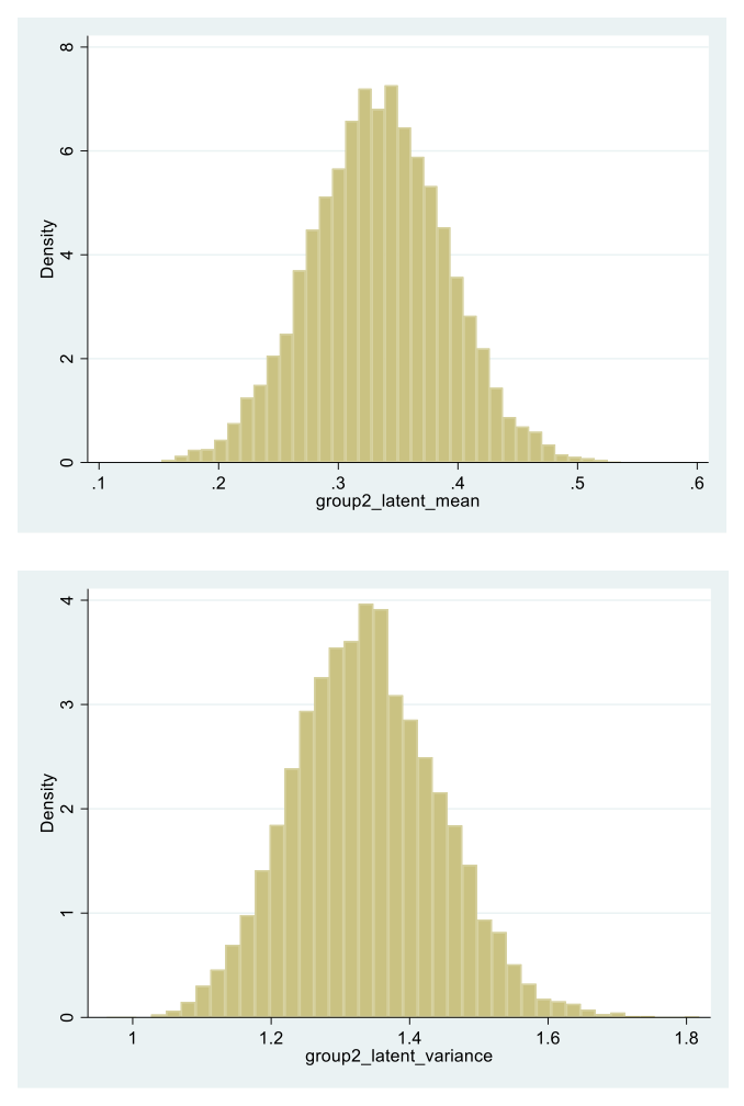
Figure 4. Histograms of the 10,000 replication sets’ latent mean and latent variance estimates (top to bottom) in Group 2 (see Equations (1) and (7), and their subsequent discussions).

As observed from the last discussed results and Figure 4, the latent mean and variance related findings show that despite the lack of MI with respect to factor loadings in the data generation process, correct latent mean and variance group difference conclusions were drawn in the unidimensionality setting (and data sets) considered in this section. These findings are consistent with the earlier made conjecture (see preceding section), and are arguably due to the facts that (a) the latent construct predictability was high and the same in both groups at the population level, and (b) the instrument component intercepts were identical across the groups.

 

Discussion and Conclusion

This paper was concerned with examination of the predictability of studied latent constructs and its population differences, when using social measurement instruments. In the multi-group setting of scale uni-dimensionality (see Equations (1)), a readily applicable procedure was outlined for estimation of the degree of group difference in latent construct predictability (GDCP). Thereby, the concepts of maximal reliability and optimal linear combination were utilized in the definition of an index of GDCP that is readily point and interval estimated using the popular LVM methodology, employing for example the software Mplus. The described approach is directly extended to the case with more than two populations by examining for instance all pairs of them. The procedure is also readily generalized to multiple abilities or constructs underlying a scale under consideration, by applying the approach (under its assumptions) with respect to each latent construct.

The outlined method of GDCP evaluation has several limitations. One is the requirement for large samples of units of analysis (oftentimes respondents or studied subjects in social science research). This is owing to the fact that its underlying estimation approach is grounded in the LVM methodology that itself is based on an asymptotic theory (Muthén, 2002). To date, there are no firm and generally applicable guidelines with respect to needed sample size in order for that theory to obtain practical relevance. A key reason is that this sample size depends on multiple factors, including number of scale components, model parameters and latent variables, the individual component psychometric quality features, and amount of missing data (fraction of missing information, for data sets with missing data). One may expect that with more reliable components, minimal number of latent variables, and arguably a larger number of scale components, the application of the discussed procedure may be more trustworthy. We encourage future research, possibly based on extensive simulation studies that go beyond the confines of this article, to address this complicated sample size query (including variation of sample size in the groups).

Secondly, the described approach is based on the assumption of a unidimensional instrument with uncorrelated errors in each population. When uni-dimensionality is violated, as indicated above application of the outlined procedure may still be possible with respect to each individual of the underlying abilities (factors), correspondingly on the assumptions made in the introductory section. Thirdly, as mentioned at the outset, this method is best employed with (approximately) continuous scale components. In case they are not normality distributed and thus the regular ML estimation method is no longer strictly applicable (Bollen, 1989), including studies with discrete scale components having at least 5-7 say possible values and preferably close to symmetric distributions, the robust maximum likelihood method or asymptotically distribution-free method can be used for model fitting and parameter estimation purposes (under the remaining assumptions of the outlined procedure; Browne, 1984; Rhemtulla, Brosseau-Liard, & Savalei, 2012). This approach is also useful with limited clustering effects, especially in cases with weak violations of normality. Relatedly, with substantial unobserved heterogeneity in studied populations with multiple latent classes, a direct application of the procedure treating each group as a single-class population can yield misleading conclusions. However, its application within individual latent classes is possible along the lines described above (especially in cases with minimal class overlap). Last but not least, it may be expected that the procedure would yield more dependable results in settings with higher MR coefficients within each of the groups.

In this context, it is worth emphasizing that our discussion in the illustration section only suggested that with high construct predictability that is very similar in the groups, it may be still (but not necessarily always or often) possible to reach trustworthy conclusions about latent population differences despite some violations of MI in the factor loadings and on the assumption of group invariant intercepts. It is worth also pointing out that such conclusions with respect to latent variances may require higher sample sizes (all else kept constant). We therefore encourage future research to address the effect of (i) MR magnitude; (ii) degree of group discrepancy in it; (iii) number of unequal loadings across groups, and degree of their inequality; (iv) sample size (both within groups and overall); and (v) number of scale components, on the dependability of the group comparison results with the outlined MR-based procedure with respect to latent means and/or variances. Last but not least, the article does not imply that the condition of the GDCP index being 0 (or close to 0) is sufficient for MI, nor do we imply that it is sufficient for measuring in all groups the same construct (see also Endnote 1). In this relation, findings of latent mean and/or latent variance group differences with the discussed method are to be substantively interpreted by subject-matter experts, or in close collaboration with them, taking correspondingly into account also the possible effect of the magnitude of GDCP, MR, and sample size.

In conclusion, this paper outlined a readily and widely applicable LVM-based procedure for point and interval estimation of an index of population differences in predictability of studied constructs, attitudes, or traits with social measurement instruments, which seems to also provide under certain conditions a potential link that is to be further explored between measurement invariance and maximal reliability. Along with maximal reliability magnitude, its group differences, and sample size considerations, the index may be suggestive of the extent to which group comparisons of underlying latent means and variances may be trustworthy in the presence of some measurement invariance violations with respect to factor loadings only (while intercepts are group invariant), as it is not infrequently found in contemporary empirical social research.

 

---

Endnotes

1. The MR is well-defined and always exists in contemporary social research with multiple populations, where the scale components are associated with positive loadings and error variances, as assumed in the article (see model (1) and its immediately following discussion).
   ↩︎
2. The lack of population differences in construct predictability is not considered or implied in this article as a sufficient condition for measuring the same substantive construct in all studied groups, or in general for meaningful and valid group comparisons in latent means and variances (see also discussion and conclusion section).
   ↩︎
3. The GDCP index Δ is well-defined and always exists in contemporary social research with multiple populations, due to both MR coefficients being positive then (and under the conditions stated in Endnote 1).
   ↩︎

Appendix 1 and 2

References

1. Agresti, A. (2018). Statistical methods for the social sciences. Upper Saddle River, NJ: Prentice-Hall.
2. Bartholomew, D. J. (1996). The statistical approach to social measurement. New York: Academic Press.
3. Bollen, K. A. (1980). Issues in the comparative measurement of political democracy. American Sociological Review, 45, 370-390.
4. Bollen, K. A. (1989). Structural equations with latent variables. New York, NY: Wiley.
5. Browne, M. W. (1984). Asymptotically distribution-free methods for the analysis of covariance structures. British Journal of Mathematical and Statistical Psychology, 37, 62-83.
6. Browne, M. W., & Cudeck, R. (1993). Alternative ways of assessing model fit. In K. A. Bollen & J. S. Long (Eds), Testing structural equation models (pp. 136-162). Newbury Park, CA: Sage.
7. Conger, A. (1980). Maximally reliable composites for unidimensional measures. Educational and Psychological Measurement, 40, 367–375.
8. Geiser, C. (2013). Data analysis with Mplus. New York, NY: Taylor & Francis.
9. Hancock, G., & Mueller, R. O. (2001). Rethinking construct reliability within latent variable systems. In R. Cudeck, S. du Toit, & D. Sörbom (Eds.), Structural equation modeling: Present and future. A festschrift in honor of Karl Jöreskog (pp. 195-216). Lincolnwood, IL: Scientific Software International.
10. Hu, L.-T., & Bentler, P. M. (1999). Cutoff criteria for fit indices in covariance structure analysis: Conventional criteria versus new alternatives. Structural Equation Modeling, 6, 1-55.
11. McDonald, R. P. (1999). Test theory. A unified treatment. Mahwah, NJ: Earlbaum.
12. Millsap, R. E. (2011). Statistical approaches to measurement invariance. New York, NY: Taylor & Francis.
13. Mulaik, S. (2009). Factor analysis. Boca Raton, FL: CRC Press.
14. Muthén, B. O. (2002). Beyond SEM: General latent variable modeling. Behaviormetrika, 29, 87-117.
15. Muthén, L. K., & Muthén, B. O. (2002). How to use a Monte Carlo study to decide on sample size and determine power. Structural Equation Modeling, 9, 599-620.
16. Muthén, L. K., & Muthén, B. O. (2025). Mplus user’s guide. Los Angeles, CA: Muthén & Muthén.
17. Rabe-Hesketh, S., & Skrondal, A. (2022). Multilevel and longitudinal modeling using Stata. College Station, TX: Stata Press.
18. Raykov, T., & Hancock, G. R. (2005). Examining change in maximal reliability for multiple-component measuring instruments. British Journal of Mathematical and Statistical Psychology, 58, 65-82.
19. Raykov, T., & Marcoulides, G. A. (2004). Using the delta method for approximate interval estimation of parametric functions in covariance structure models. Structural Equation Modeling, 11, 659-675.
20. Raykov, T., & Marcoulides, G. A. (2011). Introduction to psychometric theory. New York, NY: Taylor & Francis.
21. Raykov, T., & Marcoulides, G. A. (2018). A course in item response theory and modeling with Stata. College Station, TX: Stata Press.
22. Raykov, T., Rodenberg, C. N., & Narayanan, A. (2015). Optimal shortening of psychometric scales. Structural Equation Modeling, 22, 227-235.
23. Rhemtulla, M., Brosseau-Liard, P., & Savalei, V. (2012). When can categorical variables be treated as continuous? A comparison of robust continuous and categorical SEM estimation methods under suboptimal conditions. Psychological Methods, 18, 354 – 369.
24. Thompson, G. H. (1940). Weighting for battery reliability and prediction. British Journal of Mathematical and Statistical Psychology, 30, 357–360.