Challenges in the Treatment of Unit Nonresponse for Selected Business Surveys: A Case Study

---

Abstract

Probability sample selection procedures gift methodologists with quite a bit of control before data collection. Unfortunately, not all sample units respond and those that do will not always provide data on every questioned characteristic, which can lead to biased estimates of totals. In this paper, we focus entirely on the challenges of mitigating nonresponse bias effects in business surveys, using empirical examples from one survey to illustrate challenges common to many programs.

Keywords

missing data; weight adjustment; ratio imputation

Acknowledgement

The authors thank Laura Bechtel, William Davie Jr., Donna Hambric, Lynn Imel, Xijian Liu, Mary Mulry, and two referees for their useful comments on earlier versions of this manuscript. This paper is released to inform interested parties of research and to encourage discussion. The views expressed are those of the authors and not necessarily those of the U.S. Census Bureau.

Introduction

Probability sample selection procedures gift methodologists with quite a bit of control before data collection. At the design stage, the methodologist determines an optimal design for a given frame and characteristic(s) to ensure that the realized sample is ‘balanced…which means (the selected sample has) the same or almost the same characteristics as the whole population’ for selected items (Särndal, 2011). This control can evaporate when the survey is conducted. Not all sample units respond (unit nonresponse), and those that do will not always provide data for every item on the questionnaire (item nonresponse). Unit and item nonresponse will lead to biased estimates of totals if the respondent-based sample estimates are not adjusted. The degree of bias is a function of several factors, including the difference in respondent and nonrespondent means on the same item, the magnitude of the aggregated missing data values, and the effects of “improper“ adjustment procedures on the respondent data.

In this paper, we focus on the challenges of mitigating nonresponse bias effects in business surveys, using empirical examples from one survey to illustrate challenges common to many programs. The terms “establishment survey” and “business survey” are often used interchangeably. We use the latter term since many business surveys select companies or firms, which comprise establishments. Most business surveys publish totals such as revenue, expenditures, and employees.  Consequently, complete-case analyses are always biased.  We identify two separate but highly related estimation challenges with nonresponse in business surveys: (1) the difficulty in developing adjustment cells for nonresponse treatment  that use auxiliary variables that are predictive of both unit response and outcome and (2) the difficulty in developing appropriate nonresponse treatments for surveys that collect a large number of data items, many of which are not strongly related to key data items or to the available auxiliary data.

The General Setting: Business Populations and Business Data

Economic data generally have very different characteristics from their household counterparts. First, business populations are highly skewed, i.e. the majority of a tabulated total in a given industry comes from a small number of large units. Consequently, business surveys often employ single stage samples with highly stratified designs that include the “largest” cases with certainty and sample the remaining cases.  Thus sampled cases with large design weights may often contribute very little to the overall tabulated totals.

An efficient highly stratified design requires that within-strata means are the same, and the between-strata means are different (Lohr, 2010, Ch.3).  For this to happen, the unit measure of size (MOS) variable used for stratification must be highly positively correlated with the survey’s characteristic(s) of interest. However, it is possible for a given characteristic to have no statistical relationship with unit size.  For example, the frame MOS could be total receipts for the business, but an important characteristic of interest could be electrical consumption.  Furthermore, although business populations are highly positively skewed, not all business characteristics are strictly positive (e.g.  income, profit/loss).

Not all sampled units respond.  To account for this nonresponse, the survey designers partition the population into P disjoint adjustment cells using x_p, a vector of auxiliary categorical variables available for all units. Each adjustment cell contains n_p units, of which r_p respond. Nonresponse adjustment procedures are performed within adjustment cell, with the assumption that the respondents comprise a random subsample within the nonresponse adjustment cells.

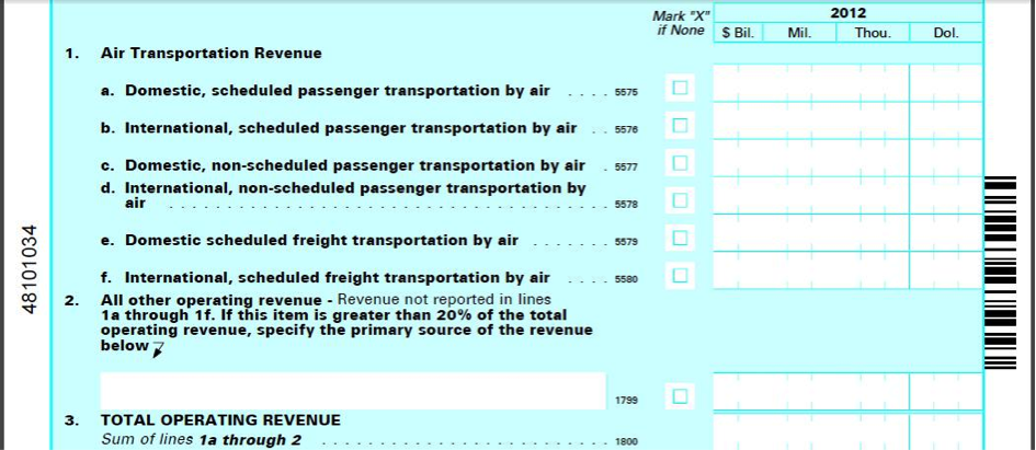
 Many business programs collect detail items – groups of items that sum up to their respective totals.  The total and associated details items are referred to together as “balance complexes” (Sigman and Wagner, 1997). All survey participants are asked to provide values for the key items (hereafter referred to as “totals”), whereas the type of requested details requested can vary. For example, Figure 1 presents the balance complex included on the Service Annual Survey (SAS) questionnaire mailed to companies that operate in the airline industry.  [The SAS population comprises several industries]. The information requested in lines 1a through 2 are details that are only requested from sampled units that operate in the airline industry (and are referred to herafter as ‘detail items’), and the information requested in line 3 is collected from all units that are sampled in the SAS.

Figure 1: Sample Balance Complex from the Services Annual Survey (Transportation Sector)

 

Data collection and nonresponse adjustment for the total items are much less problematic than for the detail items because companies are usually able to proportion out their “bottom line” total items. Moreover, alternative data are often available for substitution or validation of these items.  In contrast, with smaller units, the requested detail level data may not be available from all respondents, and auxiliary data are generally not available (Willimack and Nichols, 2010).

Furthermore, the larger units are more likely to provide response data than are the smaller units. First, the smaller units may not keep track of all of the requested data items (Willimack and Nichols, 2010) or may perceive the response burden as being quite high (Bavdaž 2010).  Second, operational procedures increase the likelihood of obtaining valid response from large units.  Analyst procedures in business surveys are designed to improve the quality of published totals. This is best accomplished by unit nonresponse follow-up of the large cases expected to contribute substantially to the estimate, followed by intensive analyst research for auxiliary data sources such as publicly available financial reports to replace imputed values with equivalent data (Thompson and Oliver, 2012). This approach works well for the key survey totals items, where alternative data are available for substitution or validation, but not for the detail items.

Frequently Used Adjustment Procedures for Unit and Item Nonresponse

There are two treatments for unit and item nonresponse:  adjustment cell weighting and imputation.  In household surveys, where there is generally little or no information corresponding to the missing data from the sampled units, adjustment weighting – which increases the sampling weights of the respondents to represent the nonrespondents – is the only legitimate option (Kalton and Kaspryzk, 1986).  In business surveys, imputation can be as appealing as weight adjustment for treating unit nonresponse, especially when valid data from the same sample unit are often available for direct substitution. Indeed, Beaumont et al (2011) prove that such auxiliary variable imputation can yield identical variances as those obtained from the full response data. In contrast to weighting, imputation is performed by item, using a hierarchy that imputes items in a pre-specified sequence determined by the expected reliability of available imputation models [Note: hot deck imputation and certain Bayesian models are exceptions to this univariate procedure but are not further discussed in this paper as their usage is fairly rare with business surveys]. This approach allows great flexibility and preserves the expected cell totals, but does not preserve multivariate relationships between items.

In our setting, the business survey has a random sample of size s that has been partitioned into P disjoint unit nonresponse adjustment cells, indexed by p. In each imputation cell p, s_p,r units respond and s_p,nr units do not.  Thus, survey data are available for the variable of interest y from the s_p,r responding units. A vector of auxiliary variables x exists for all the sampled units (respondents and nonrespondents). Under complete response, the population total Y would be estimated as where w_j is a weight associated with unit j (usually the inverse probability of selection).  The imputed estimator of the population total for characteristic y is given by

   

where is the imputed value obtained for nonrespondent unit in adjustment cell .

Our case study considers three commonly used imputation models. Each model can be re-expressed as an adjustment-to-sample weighting estimators, as described in Kalton and Flores-Cervantes (2003). Here, the weighted estimator of the population total for characteristic y is given by

   

where is a weight adjustment factor to account for unit nonresponse, is a unit response indicator, and is the nonresponse adjusted weight for unit in adjustment cell under procedure . The adjusted weight will be a positive value for respondents and will equal zero otherwise.

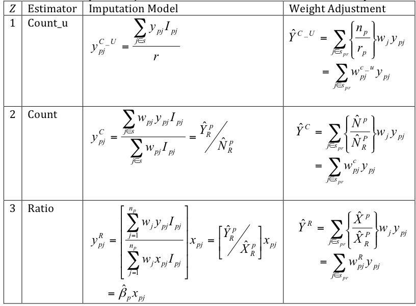
Table 1 presents the three imputation/weighting procedures. The count_u procedure imputes the weighted average value in the imputation cell for the missing value.  This is equivalent to adjusting the respondent units’ final weights by the weighted inverse response rate (Oh and Scheuren, 1983).

The count procedure uses an unweighted mean for imputation, which is equivalent to multiplying the respondent units’ final weights by an unweighted inverse response rate (see Särndal and Lundström, 2005, Chapter 7.3, and Little and Vartivarian, 2005).

If the probability of unit nonresponse does not depend on the values of the observed characteristic y, then the data are missing at random (MAR) as defined in Rubin (1976). Under this assumption, the probability of response in each adjustment cell p is a constant, and the “inverse response rate” adjustment to the design weights produces an “unbiased” total from the respondent data. These adjustments are simple to compute, but the additional stage of weighting increases the variance (Kish, 1992); Kalton and Flores-Cervantez, 2003; Little and Vartivarian, 2005).

With business survey data, the probability of response is often related to unit size, and the uniform response assumption (i.e., MAR) is not realistic.  Shao and Thompson (2009) describe the more general covariate-dependent response mechanism, which allows the probability of response to depend on a strictly positive auxiliary variable x such as the MOS. Under this response model, the count adjustments described in the paragraph above do not mitigate the nonresponse bias and can only increase the sampling variance (Little and Vartivarian, 2005).

The ratio procedure predicts a value for the missing y with the no-intercept linear regression regression model described by . The weighted model incorporates unequal sampling and unit size in the parameter estimation, and the weighted least squares estimate is the best linear unbiased estimator of β under this model. Note that Särndal and Lundström (2010) recommend the inclusion of an intercept, but we have found that the intercept is non-significant in many business data sets (ex., businesses with no employees have no payroll).  If the covariate-dependent response mechanism is appropriate and the auxiliary variable x is used in the ratio model or is highly correlated with the ratio model, then the ratio adjusted estimates described in Table 1 will have improved precision over the correponding count adjusted estimates. If the prediction model is not valid or if the strength of association between x and y is weak, then the bias induced by the ratio estimator increases the MSE over the other reweighted estimates.  This is more likely to occur with the detail items than with the total items.

Table 1: Nonresponse Adjusted Estimators Considered in the Case Study

Hereafter, as in Table 1, we use the term ‘imputation model’ to describe the formula used to obtain an imputed (replacement) value for the missing y and the term ‘imputation parameter’ to describe data-driven estimates obtained from respondent values to compute these replacement values (the weighted or unweighted sample mean or ).

The Service Annual Survey (SAS)

For the remainder of the report, we discuss the analysis of the nonresponse adjustment procedures for the Service Annual Survey (SAS).  The SAS is a mandatory survey of approximately 70,000 employer businesses having one or more establishments located in the U.S. that provide services to individuals, businesses, and governments, identified by North American Industry Classification Series (NAICS) system code on the sampling frame. We examine the SAS sections covering the transportation and health industries (SAS-T and SAS-H, respectively). Information on the SAS design and methodology is available at http://www.census.gov/services/sas/about_the_surveys.html.

The SAS uses a stratified random sample. Companies are stratified by their major kind of business (industry), then are further sub-stratified by estimated annual receipts or revenue. All companies with total receipts above applicable size cutoffs for each kind of business are included in the survey as part of the certainty stratum. Within each noncertainty size stratum, a simple random sample of employer identification numbers (EINs) is selected without replacement. Thus, the sampling units are either companies or EINs.  The initial sample is updated quarterly to reflect births and deaths.

The key items collected by SAS are total revenue and total expenses, both of which are totals in balances complexes. The revenue detail items vary by industry within sector. Expense detail items are primarily the same for all sectors, with an occasional additional expense detail or two collected for select industries. Total payroll is collected in all sectors as a detail item associated with expenses. For editing and imputation, payroll is treated as a total item, as auxiliary administrative data are available.  Imputation is used to account for both unit and item nonresponse. Auxiliary variable and historic trend imputation (which uses survey data from the same unit in a prior collection period) are preferred for revenue, expenses, and payroll.  Otherwise, SAS-H and SAS-T utilize the trend and auxiliary ratio imputation models, where the trend module predicts a current period value of y from a prior period value and the auxiliary model uses a different auxiliary variable obtained from the same unit and collection period.

The imputation cells for SAS are six-digit industry (NAICS) code cross-classified by tax-exempt status. Unlike the sampling strata definitions, the imputation cells do not account for unit size, and imputation parameters use certainty and (weighted) noncertainty units within the same cell. The imputation base for the ratio imputation parameters is restricted to complete respondent data, subject to outlier detection and treatment.

Response Propensity Analysis

Response propensity modeling uses logistic regression analysis to determine sets of explanatory covariates related to unit response. Separately examining the SAS-T and SAS-H data, we used the SAS SURVEYLOGISTIC procedure[i] to fit two logistic regression models: (1) a simple model that used only the existing imputation cells as independent variables; and (2) a nested model that also included the continuous MOS variable as a covariate. The logistic regression analysis therefore examines whether the categorical variables used to form adjustment cells are predictive of unit nonresponse and to check if other variables are missing in the construction of the adjustment cell.

We tested the goodness-of-fit hypothesis of each fitted model. All were significant, so we examined the marginal test results for individual imputation cells for cells with good fits. Rejecting the goodness-of-fit null hypothesis provides evidence that at least one of the variables used to construct adjustment cells are related to response propensity. Examining the marginal results highlights individual imputation cells where there may be a missing predictor.

Figure 2 presents side-by-side bubble plots summarizing the logistic regression results for SAS-H.  Figure 3 presents the corresponding counts for SAS-T.

Figure 2:  Logistic Regression Results for SAS-H. Each dot represents number of significant marginal test results for an individual imputation cell, with the number of significant tests indicated on the y-axis. A strongly predictive model should have significant results in at least four of the six studied years.

 

Figure 3: Logistic Regression Results for SAS-T

For both programs, the logistic regression analysis provides evidence that the industry/tax status categories used to form adjustment cells are not strongly related to response propensity. Including the continuous nested MOS covariate in the SAS-T model improves the predictions, although there is no evidence that this is the case with SAS-H.

Clearly, the existing sets of categorical variables used to form imputation cells for SAS-T are inadequate for mitigating unit nonresponse. Initially, we considered using the sampling strata as adjustment cells.  However, a high proportion of strata contained fewer than five units because of the highly stratified design and the limited number of large companies and large tax-entities in the sampling universe.

Unit Response Rate Comparisons

With SAS, certainty status is directly related to response propensity through the analyst follow-up procedures. Särndal and Lundström (2005) recommend exploring whether there is a sytematic difference in response propensities on a single category by comparing their unit response rates (URR) in the same imputation cell. In the Economic Directorate of the U.S. Census Bureau, the URR is the ratio of units that reported valid data to the total number of eligible units, computed without survey weights (Thompson and Oliver 2012).

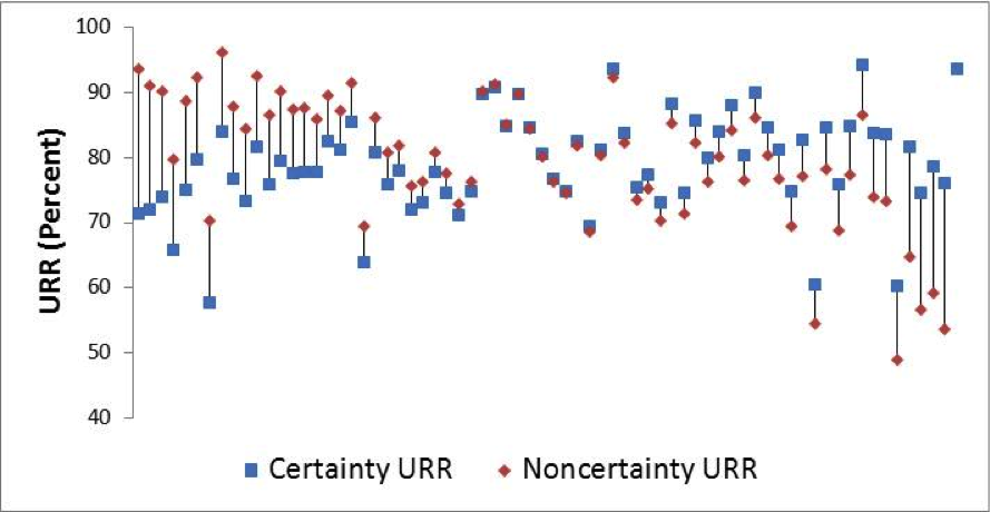
Figure 4 presents the average URR (across the six years) for each SAS-H imputation cell, with blue squares presenting the certainty-unit URR, and the red squares presenting the noncertainty-unit URR in the same imputation cells. In the majority of cases, the certainty and noncertainty URRs within the same cell are dissimilar, although the direction of the difference is not consistent.

Figure 5 presents the corresponding measures for SAS-T. As with SAS-H, the URRs within the same imputation cell clearly differ by certainty status. In contrast to the SAS-H results, there is a very clear pattern within the SAS-T cells, where the unit response rates for certainty units are generally higher than the corresponding noncertainty measures.

Figure 4: Average URR by Certainty Status within Imputation Cell (SAS-H)

Figure 5: Average URR by Certainty Status within Imputation Cell (SAS-T)

The transportation sector tends to have a few very large units (businesses) in each industry, with the remaining units being fairly homogeneous in size, and the analysts attempt to obtain complete data from all certainty cases. In contrast, the unit size within the health sector is much more variable, and the SAS-H sample is much more highly stratified. Analysts must obtain valid responses from certainty and “large” noncertainty units, so the response rate pattern is not as consistent.

 Alternative Weighting Comparisons

The earlier analysis indicates that the studied programs’ imputation cells fail to satisfy the MAR assumption. That said, if the degree of nonresponse bias in the studied estimates is small, then this might not be of strong concern. Groves and Brick (2005) propose evaluating the magnitude of the nonresponse bias by altering the estimation weights and using the various weights to construct different estimates. If the difference between the estimates is trivial, there is evidence that the nonresponse bias may not be large.

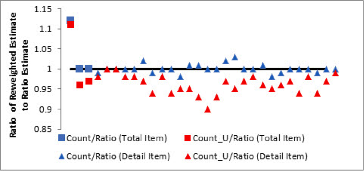
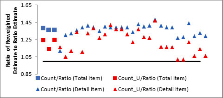
To vary the weights, we re-express the ratio imputation models as ratio reweighting models as shown in Table 1, and likewise re-express the presented alternative mean imputation models as the reweighted count and count_u estimators. We computed these three alternatively weighted estimates for each item by publication industry in our six years of data.  For each item, we obtain the ratio of the count and count_u weighted estimates to the ratio estimates (the current imputation method).  Figures 6 and 7 presents the “double-averaged” estimate ratios[ii] for the SAS-H and SAS-T items.

Figure 6: SAS-H Reweighted Estimates (Averaged Within Statistical Period and Across Industry). In these plots, the total items (receipts, expenditures, and payroll) are represented by squares, and the various detail items are represented by circles. Each graph includes a horizontal asymptote at y = 1 to indicate the estimate ratios that are essentially unaffected by reweighting.

Figure 7: SAS-T Reweighted Estimates (Averaged Within Statistical Period and Across Industry)

With SAS-H, the count and ratio estimates are very close, regardless of whether the collected item is a total or a detail.  However, the differences between the count_u and ratio estimates are more pronounced. The SAS-H results are “different enough” to merit some concern about unmitigated nonresponse bias, whereas the SAS-T results are much more conclusive. The differences among the three sets of SAS-T estimates are very pronounced, indicating estimation effects caused entirely by changes in adjustment methodology.

These analyses highlight issues with unit nonresponse in business data and challenges in remediating these issues. First, the URR is not necessarily a good measure of representativeness of the sample (Peytcheva and Groves, 2009).  In our case study, the majority of the URRs are at an acceptable level, but the other analyses show that the larger units respond at a higher rate than the smaller units. By partitioning the existing imputation cells by size categories, we can likely reduce the nonresponse bias. However, there are insufficient numbers of sampled units in the sampling strata to use them as adjustment cells, and the small number of “large” units makes it challenging to subdivide the existing cells. In the future, it may be possible to develop strata collapsing procedures during the survey design stage.

Evaluation of the Prediction (Imputation) Models

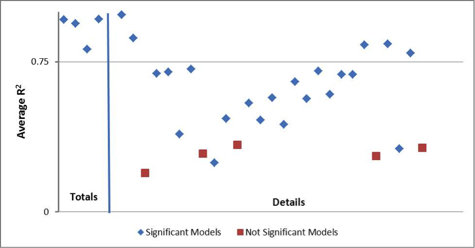
The SAS uses the ratio imputation model from Table 1 when auxiliary data or historic data from the same unit are not available: Matthews (2011) and Nelson (2011) provides information on each item’s imputation model.  To assess the imputation models’ predictive properties, we fit each regression imputation model within the currently used imputation cells with the SAS SURVEYREG procedure, again excluding certainty cases.  Figures 8 and 9 summarize the regression analysis results for SAS-H and SAS-T, respectively. These figures plot the average R² value from each model. We consider any R² value above y = 0.75 would to be strongly predictive. The total items (receipts, expenses, and payroll) and detail items are separated by a vertical asymptote and are annotated as such in the Figures.

Figure 8: Regression Analysis Results for Item Imputation Models (SAS-H). A blue diamond indicates a consistently significant model (at α = 0.10) and a red square indicates the reverse.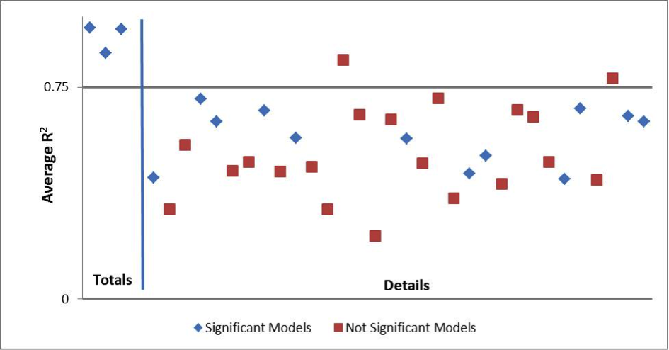

Figure 9:  Regression Analysis Results for Item Imputation Models (SAS-T)

In both programs, the models that predict the totals items are strongly predictive. However, the models used to impute the detail items are generally not.  Hence model-imputation for totals is appropriate, but rarely used due to the availability of alternative data sources such as administrative or historic data, and model-imputation for details is not necessarily appropriate, but is frequently employed.

Of course, the effectiveness of a ratio imputation model for correcting nonresponse bias is highly dependent on the availability of data for parameter estimation. For SAS, the respondent units must provide valid values for either revenue or expenses, not necessarily both. On the average, the item response rates for SAS are quite low – generally between 50 to 60 percent for totals and between 40 to 60 percent for detail items, regardless of the sector.  Furthermore, the unit size does not appear to be a factor in item nonresponse: item response rates computed separately for certainty and noncertainty units in the same industry tend to be very close.

The earlier analyses provided indications that the SAS imputation cells should be further subdivided to account for unit size. If the imputation parameters are approximately the same for each unit size category within an imputation cell, then the “dominance” of the large cases would not influence the predictions. On the other hand, if imputation parameters did differ by unit size within industry, then the adjustment strategy being used is inducing systematic bias.

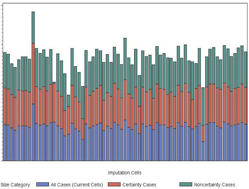
To investigate this, we obtained the ratio imputation parameters in the current imputation cells, then refit the same regression models with more refined industry cells (splitting the industry data into certainty and and noncertainty components). Figure 10 presents stacked imputation parameters from the ratio model that uses expenditures to predict revenue using 2010 SAS-H data. Each bar represents a set of regression imputation parameters from the original imputation cell.

Figure 10: Ratio Imputation Parameters for Revenue/Expenses (SAS-H 2010). The blue bar is the regression parameter obtained using all units in the industry, the red bar is the regression parameter obtained using only the certainty units, and the green bar is the regression parameter obtained from the noncertainty units.

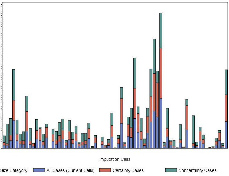
In Figure 10, all of the imputation parameters are approximately the same, with a few exceptions. This pattern repeats in the SAS-H and SAS-T data for all data collection years.  However, this is a ratio of two well-reported totals items that are generally imputed with auxiliary data. When we examine a similar plot for a typical SAS-H detail item, the situation is quite different, as shown in Figure 11.

Figure 11: Ratio Parameters for a Typical SAS-H Detail Item Ratio

Here, the imputation parameters computed from the certainty cases have almost exactly the same value as the parameters computed from the complete data in the imputation cell, and the imputation parameters for the noncertainty units are each quite different. In short, the ratio imputation model causes all imputed units to resemble the certainty units. Similar plots are available for all ratio imputation parameters upon request, but are not included for brevity. However, the vast majority of imputation model analyses for the detail items demonstrated similar patterns.

Finally, we examine the effect of choice of imputation cell by item, given a nonresponse adjustment method.  Figures 12 and 13 shows “double-average” ratios of estimates computed using the same weights with different adjustment cells, comparing estimates obtained using the existing cells subdivided by certainty status (more refined parameters) to those obtained from the currently used imputation cells. For SAS-T, the totals do not vary much, regardless of adjustment method, and many of the detail items that were imputed with the ratio model maintain similar levels as well. With SAS-H, the choice of adjustment cell has a very large impact on the estimate levels, regardless of whether the item is a total or a detail.

Recall that the SAS-T sampled unit population is fairly homogeneous in size, in contrast to the SAS-H sampled unit population. For SAS-T, the choice of adjustment cell is the most important factor in nonresponse bias mitigation. In this population, the ratio imputation models (which incorporate unit size in the parameter estimation) are quite good for totals, but not so for details.  With SAS-H, it is not immediately clear which factor (adjustment cell or adjustment method) is more important in nonresponse bias mitigation. Although it appears that unit size is not strongly related to response propensity for this population, it is also apparent that unit size is very related to prediction for the key totals. Unfortunately, this strong relationship is not true for the SAS-H details.

Figure 12: Comparison of Alternatively Weighted Estimates by Imputation Cell (SAS-H)

 

Figure 13: Comparison of Alternatively Weighted Estimates by Imputation Cell (SAS-T)

In SAS, imputation is performed independently in each adjustment cell. Consequently, the improper adjustment bias is aggregated, and it is impossible to determine what the cumulative effects of the bias are (if it exists). Besides, there is a data quality cost. Because all imputed items maintain the certainty-unit ratios, the imputed individual micro-data are not realistic, and all multivariate item relationships are lost. Furthermore, there is little evidence to validate the ratio models used for the detail items.

Discussion

This case study highlights several of the major challenges that business surveys encounter in addressing unit nonresponse.  Respondents often do not comprise a random subsample, as larger units are more likely to provide data than smaller units.  This phenomenon is an artifact of several factors, including the perceived benefits of the survey by the business community and the existing analyst nonresponse follow-up procedure, which focuses on obtaining the most accurate estimated totals.

Developing a set of adjustment cells that satisfy the most common ignorable response mechanism conditions and contain sufficient respondents is equally challenging, as there are considerably fewer “large” units in the population than small units.  Finally, there are data collection and quality challenges, as several of the detail items that the survey would like to collect may not be available from the majority of the sampled units.  Again, the respondent sample size issues for the detail items are compounded by collecting different sets of detail items by industry or sector.

For SAS, we hope to improve existing adjustment techniques by refining the adjustment cells to account for missing covariates simply by subdividing the cells into certainty and noncertainty components.  This should not detrimentally affect the quality of the estimates of the totals items, and may improve the ratio imputation procedures for the details.  However, especially with low item response, we have no way of validating the latter.  Simply put, we need data.

There are several excellent references on the use of adaptive or responsive designs to reduce the incidence of nonresponse bias by monitoring data collection and adapting procedures on a flow basis, utilizing different nonresponse follow-up strategies depending on response propensity (Groves and Heeringa, 2009; Laflamme et al, 2008), focussing on small businesses.  This adaptive strategy could provide the information needed to learn about the missing data characteristics and would yield more statistically defensible nonresponse bias-amelioration procedures.

References

1. Andridge, R.R. and Little, R.J.A. (2011).  Proxy Pattern-Mixture Analysis for Survey Nonresponse. Journal of Official Statistics, 27, pp. 153-180.
2. Bavdaž, M. (2010). The Multidimensional Integral Business Survey Response Model.  Survey Methodology, 1, pp. 81-93.
3. Beaumont, J.F., Haziza, D., and Bocci, C. (2011). On Variance Imputation Under Auxiliary Variable Imputation in Sample Surveys.  Statistica Sinica, 21, pp. 515-537.
4. Groves, R. and Brick, J. (2005). Practical Tools for Nonresponse Bias Studies. Joint Program in Survey Methodology course notes.
5. Groves, R. and Heeringa, S. (2006).  Responsive Design for Household Surveys:  Tools for Actively Controlling Survey Errors and Costs. Journal of the Royal Statistical Society, Series A, 169, pp. 439-457.
6. Kalton, G. and Flores-Cervantes, I. (2003). Weighting Methods. Journal of Official Statistics, 19, pp. 81-97.
7. Kalton, G. and Kasprzyk, D. (1986).  The Treatment of Missing Survey Data. Survey Methodololgy, 12, pp. 1 -16.
8. Kish, L. (1992). Weighting for Unequal P_i,  Journal of Official Statistics, 8, pp.183-200.
9. Laflamme, F., Maydan, M., and Miller, A. (2008). Using Paradata to Actively Manage Data Collection Survey Process. Proceedings of the Section on Survey Research Methods, American Statistical Association.
10. Little, R.J.A. and Rubin, D.R. (2002). Statistical Analysis with Missing Data. New York:  John Wiley and Sons.
11. Little, R.J.A. and Vartivarian, S. (2005). Does Weighting for Nonresponse Increase the Variance of Survey Means? Survey Methodology, 31, pp. 161-168.
12. Lohr, S.L. (2010). Sampling:  Design and Analysis (2^nd Edition). Boston:  Brooks/Cole.
13. Matthews, B. (2011).  StEPS Imputation Specifications for the Health Portion of the 2010 Service Annual Survey (SAS-H). U.S. Census Bureau internal memorandum, EDMS #7526, available upon request.
14. Oh, H.L., and Scheuren, F.J. (1983). Weighting Adjustment of Unit Nonresponse. Incomplete Data in Sample Surveys. New York:  Academic Press, 20, 143-184.
15. Nelson, M. (2011). StEPS Imputation Specifications for the Transportation Portion of the 2010 Service Annual Survey (SAS-T). U.S. Census Bureau internal memorandum, EDMS #38537, available upon request.
16. Peytcheva, E. and Groves, R. (2009).  Using Variation in Response Rates of Demographic Subgroups and Evidence of Nonresponse Bias in Survey Estimates. Journal of Official Statistics, 25, pp. 193-201.
17. Roberts, G., Rao, J.N.K., and Kumar, S. (1987). Logistic Regression Analysis of Sample Survey Data.  Biometrika, 74, pp. 1 – 12.
18. Särndal, C.E. (2011).  The 2010 Morris Hansen Lecture: Dealing with Survey Nonresponse in Data Collection, in Estimation. Journal of Official Statistics, 27, pp. 1-21.
19. Särndal, C.E., Swenssen, B., and Wretman, J. (1992). Model Assisted Survey Sampling. New York: Springer-Verlag.
20. Särndal, C.E. and Lundström, S. (2005). Estimation in Surveys with Nonresponse. New York: John Wiley & Sons, Inc.
21. Särndal , C.-E. and Lundström , S. (2010). Design for Estimation: Identifying Auxiliary Variables to Reduce Nonresponse Bias. Survey Methodology, 36, pp. 131-144.
22. Shao, J. and Thompson, K.J. (2009).  Variance Estimation In The Presence of Nonrespondents and Certainty Strata.  Survey Methodology, 35, pp. 215-225.
23. Sigman, R.S. and Wagner, D. (1997). Algorithms for Adjusting Survey Data That Fail Balance Edits. Proceedings of the Section on Survey Research Methods, American Statistical Association.
24. Thompson, K.J. and Oliver, B.E. (2012). Response Rates in Business Surveys: Going Beyond the Usual Performance Measure. Journal of Official Statistics, 28, pp. 221-237.
25. Thompson, K.J. and Washington, K.T. (2012).  Challenges in the Treatment of Nonresponse for Selected Business Surveys. Proceedings of the Section on Survey Research Methods, American Statistical Association.
26. Willimack, D.K. and Nichols, E. (2010). A Hybrid Response Process Model for Business Surveys.  Journal of Official Statistics, 1, pp. 3-24.