The Impact of Typical Survey Weighting Adjustments on the Design Effect: A Case Study

Special issue

---

Abstract

In survey sampling, the final sample weight assigned to each sampled unit reflects different steps of weighting adjustments such as frame integration, nonresponse and calibration. The analysis of the design effects for each of these adjustments casts light on their effects on the precision of survey estimates. In this paper, we limit our scope to the Canadian Community Health Survey (CCHS), briefly describe the weighting process of this survey and examine design effects at different steps of the weighting process to quantify how the overall variability in estimates can be attributed to the complex survey design and to each of the individual adjustments in the weighting process. As expected, the results suggest that the use of unequal person-selection probabilities and the nonresponse adjustment have the most negative impact on the design effect of the CCHS while calibration and winsorization decrease the design effect and improve the precision of the estimates.

Keywords

bootstrap, complex survey design, design effect, multiple frames, weighting

Acknowledgement

The authors would like to thank Jean-François Beaumont and Sharon Wirth for their comments and suggestions that helped to improve the content of this document.

The work presented in this paper is the responsibility of the authors and does not necessarily represent the views or policies of Statistics Canada.

1. Introduction

Weighting is an essential component of a survey process. The main reason for the use of weights is to compensate for unequal selection probabilities and nonresponse bias. Kish (1992) identified seven possible reasons for weightings, such as nonresponse, frame problems and statistical adjustments like post-stratification. In general, the first step in estimation is assigning a base weight, the inverses of the inclusion probabilities, to each sampled unit. Base weights are then adjusted for other sources of weighting. Hence in complex surveys, final sample weights consist of several steps of weighting adjustments. Early work in this area examined the effects of unequal weighting, stratification and clustering on the efficiency of design under certain assumptions. In particular, Kish (1987) proposed an indirect approach that estimates the design effect component incorporating the effect of unequal weighting. The concept of design effect will be clearly defined later.

In this paper we focus on the Canadian Community Health Survey (CCHS) and estimate its design effect at different steps of the weighting process. In Section 2, we briefly review the definition and use of design effect with special emphasis on the design effect decomposition. In Section 3, we discuss the sampling design and weighting process of the CCHS. Subsequently, in section 4, we compute the design effects of three variables at different steps of weighting adjustments and discuss the variability of design after each adjustment. Finally, we summarize our discussion in Section 5. The findings help guide possible modifications to lower the overall design effect and improve the effective sample size.

2. A Brief Review on Definition of Design Effect

Design effect is widely used to compare the efficiency of survey designs and to develop sampling designs. Kish (1965) defined the design effect as the ratio of the sampling variance of an estimator under a given design to the sampling variance of an estimator under simple random sampling (SRS) of the same sample size. In practice, an estimate of the design effect is calculated using the corresponding variance estimators for the sample data set (Lehtonen and Pahkinen, 2004, p.15).

   

where subscript refers to the actual sampling design and denotes the estimator of a population parameter . For complex designs, the estimation of the sample variance, , is complicated and it is often computed using replication techniques, such as bootstrap and Jackknife.

If the design effect is less than one, this indicates that the sample design leads to estimates with smaller variance than under an SRS design, therefore it is more efficient. Similarly, when design effect values are greater than one, the sample design is less efficient than an SRS design. The design effect has an impact on the sample size required to do an analysis. The larger the design effect, the more sample required to obtain the same precision of an estimate as would have been obtained under an SRS design. This is why small design effects are desired when developing a sampling design.

Complex sample designs involve several design components such as stratification, clustering and unequal weighting. The impact of these components on the efficiency of design can be assessed through decomposition of design effects. Assuming that finite population correction (fpc) factor can be ignored, Kish (1987) proposed the design effect decomposition as a function of two independent components associated with clustering and unequal weighting.

   

where denotes the relative variance of the sample weights, is the mean of cluster size and is the intra-class correlation coefficient.

Kish (1992) presented another formula for expressing the first component of the above formula, the design effect due to unequal weighting, for a sample mean:

   

where is the final sample weights of the unit in the sample and .

Kish’s decomposition method received much attention by survey samplers. Gabler et al. (1999) provided a model-based justification for Kish’s formula. Kalton et al.,(2005), and Lehtonen and Pahkinen (2004) provided the analytical evaluation of design effects and examined separately the design effects resulting from proportionate and disproportionate stratification, clustering and unequal weighting adjustments. Park et al. (2003) extended Kish’s decomposition and included the effect of stratification.

While decomposition of the design effect can provide an approximate measure of the impact of unequal weighting due to nonresponse adjustment, it is not a good approximation when weights are post-stratified or calibrated to known totals (Lê et al., 2002). Moreover, the above equations are true under certain assumptions. In particular, the later equation depends on the assumption of equal strata means and constant within-stratum variances (Lê et al., 2002). Some of these assumptions do not hold in practice.

Considering the limitation of decomposition method in practice, we empirically evaluate the design effect of the Canadian Community Health Survey (CCHS) at different steps of the weighting process.

3. The Canadian Community Health Survey

The Canadian Community Health Survey (CCHS) is a cross-sectional survey that collects information related to health status, health care utilization and health determinants for the Canadian population. The target population of the CCHS is all persons aged 12 years and over living in private dwellings across Canada. The CCHS relies upon a large sample of respondents and is designed to provide reliable estimates at the health region (HR) level. Health regions refer to health administrative areas with population sizes varying from about 10,000 to 2,250,000 persons aged 12 and over. To provide reliable HR-level estimates, a sample of 65,000 respondents is selected annually. A multi-stage sample allocation strategy gives relatively equal importance to the HRs and the provinces. In the first step, the sample is allocated among the provinces according to the size of their respective populations and the number of HRs they contain. Each province’s sample is then allocated among its HRs proportionally to the square root of the population in each HR.

The CCHS uses three sampling frames to select a sample of households (Béland et al., 2005). 49.5% of the sample of households came from an area frame, 49.5% came from a list frame of telephone numbers and the remaining 1% came from a Random Digit Dialing (RDD) sampling frame. The area frame used by the CCHS is the one designed for the Canadian Labor Force Survey (LFS). The LFS design is a multi-stage stratified cluster design in which the dwelling is the final sampling unit. In the first stage, homogeneous strata are formed and independent samples of clusters are drawn from each stratum. In the second stage, dwelling lists are prepared for each cluster and dwellings are selected from these lists. The CCHS basically follows the LFS sampling design with health regions generally forming the strata. The telephone list frame is the InfoDirect list, an external administrative database of names, addresses and telephone numbers from telephone directories in Canada. Within each stratum (generally the HR), the required number of telephone numbers is selected using a Simple Random Sampling (SRS) design. The units belonging to the telephone list frame and the RDD are interviewed using computer assisted telephone interviewing (CATI), and area frame units are interviewed using computer assisted personal interviewing (CAPI). The CCHS interviews (CAPI or CATI) are done in two parts. First, a knowledgeable household member is asked to provide basic demographic information on all residents of the dwelling (roster of the household). Then, one member of the household is selected using unequal probabilities of selection.

Given this complex survey design, several steps of weighting adjustments are required. Sarafin et al. (2007) presented a summary of the weighting strategy providing more explanations on the reason and nature of each adjustment. Figure 1 was extracted from that paper and summarizes the steps.

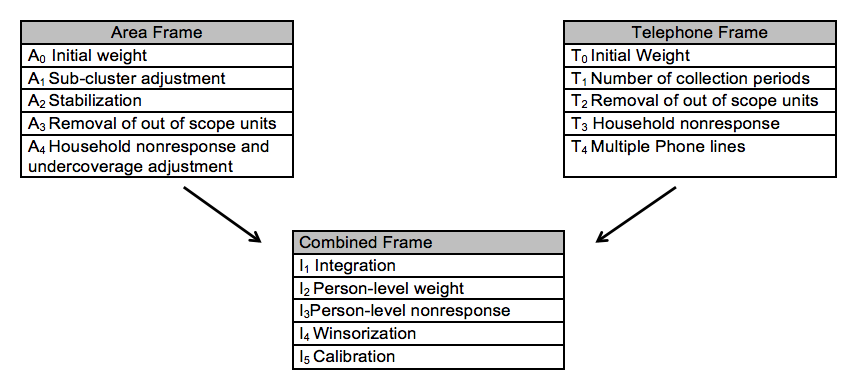
Figure 1: Weighting process

4. Evaluating the Design Effect at Different Steps of the Weighting Process

In order to evaluate the design effect at different steps of the process, we need to have variables that are available at the household level. We choose variables with different prevalence rates (i.e., proportions) to get more exhaustive results. The variables of interest are:

• Households with at least one “child” (national prevalence at 20%)
• Households with one or two “kids” (national prevalence at 10%)
• Households with five members (national prevalence at 5%)

It should be mentioned that “child” is defined as a person who is less than 12 years old, and “Kid” refers to a person living in a household whose age is less than 6 years.

The design effects of these variables are calculated at the health region level, which is the main domain of interest, after each of the following weighting adjustments.  The codes are based on Diagram 1:

1. Removal of out-of-scope units- A₃ and T₂,
2. Household nonresponse- A₄ andT₃,
3. Integration- I₁,
4. Person-level weight- I₂,
5. Person-level nonresponse- I₃,
6. Winsorization- I₄ and
7. Calibration- I₅.

To derive design effects, variances under the CCHS design are calculated using the bootstrap method. An extended version of the proposed bootstrap method by Rao, Wu and Yue (1992) has been used by the CCHS since the survey’s first occurrence in 2001. Yeo, Mantel and Liu (1999) described the adaption of the method to the particularity of Statistics Canada’s National Population Health Survey, which is the predecessor to the CCHS and used a similar methodology.

By using the bootstrap method, all of the design aspects that we are interested in, up to and including the weighting step of interest, are included in the design variance estimate. The role of bootstrap method and its impact on the estimates of design effects is discussed in sub-section 4.9.  The estimates of design effects are produced using BOOTVAR, which is a set of SAS macros (also available for SPSS) developed at Statistics Canada to estimate variances using the bootstrap method.

The design effects are calculated at health region level (112 health regions) for different steps of weighting. In other words, for each variable 112 design effects are estimated. In each sub-section below, a short description of the weight adjustment is given followed by a box-plot diagram that shows the estimates of design effect for 112 health regions  at that particular step of weighting for variables of interest. In the following sub-sections, we use the term “design effect distribution” to refer to estimates of design effect across 112 health regions. This should not be confused with the probability distribution.

4.1 Removal of out-of-scope units (Steps A₃ and T₂)

The first step in evaluating the CCHS process is to closely examine the effect of the sampling design on the area and telephone frames. The weights obtained just after the out-of-scope removal is chosen for this evaluation partly because of practical reasons.

During collection, some sampled dwellings are found to be out-of-scope. For example dwellings that are demolished, under construction or institutions are identified as being out-of-scope in the area frame while numbers that are out of order or for business are out-of-scope on the telephone frame. These units and their associated weights are removed from sample. In 2010, the rate of out-of-scope units in the area frame and the telephone frame were 15.1 % and 14.9 %, respectively.

At this step we are interested in calculating estimates that include both responding and nonresponding households. However, at this point in the process the CCHS data files would only contain information on the variables of interest from responding households. Therefore, data for the non-respondent households are imputed at this step. The non-respondent households are imputed based on the prevalence rate of the variables (p_i) at the CCHS stratum level. The imputed variable and the bootstrap weights at this point are used as input into Bootvar. Figure 2 and Figure 3 present the design effect distribution at the HR level after removal of out of scope in the area frame and in the telephone frame.

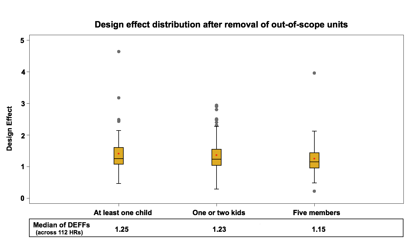
Figure 2: Design effect distribution (across 112 HRs) after removal of out of scope units in the area frame

The median of health region design effects for each variable fluctuate around 1.2 for the area frame and around 1 for the telephone frame. These results are expected since the telephone frame sampling design is a simple random sampling process within each stratum while the sampling design of the area frame is a multi-stage stratified cluster design.

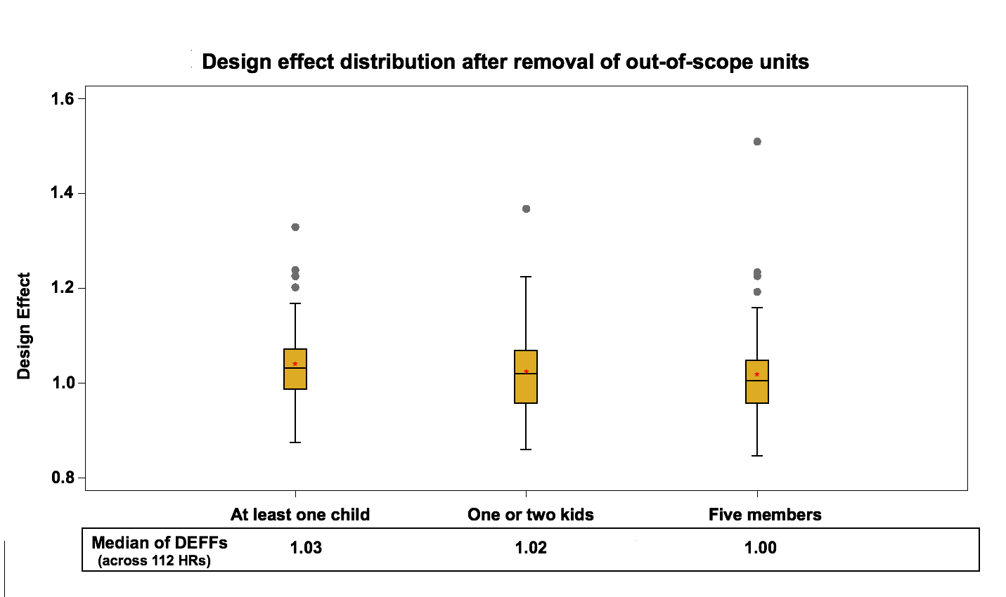
Figure 3: Design effect distribution (across 112 HRs) after removal of out of scope units in the telephone frame

The results reflect the effect of the sample selection design on the variance. They represent the starting point for the weighting adjustments that will be evaluated in the next steps.

4.2 Household Nonresponse (Steps A₄ and T₃)

Household nonresponse occurs when a household refuses to participate in the survey or cannot be reached for an interview. In 2010, out of 88410 in-scope units, 17095 households did not accept to participate in the survey resulting in an overall household-level non-response rate of 19.3%.These units are removed from the sample and their weights are redistributed to responding households within response homogeneity groups. These groups are created based on logistic regression models where the sample is divided into groups with similar response propensities within a province. The following adjustment factors are calculated within each response group:

Area Frame:

   

Telephone Frame:

   

The weights after steps A3 and T2 of responding households are multiplied by these factors to produce the weights A4 and T3.

To evaluate the effect of the household nonresponse adjustment, we compute the design effect just before the integration step. It should be noted that before the integration step, we have the effect of “Multiple Phone lines- T4” adjustment in the telephone frame which should only have a small impact on the design effect since it affects very few units. This step is not considered in this study. An adjustment in the area frame is also done before the integration to account for the under-coverage. The area frame has about 12 % households’ under-coverage using the current LFS design. In order to deal with this frame defect, a post-stratification adjustment is applied at the HR level using the most up-to-date household counts. This adjustment has no impact on the design effect at the HR level since it is a ratio adjustment that does not affect the estimates of proportions or their variances. Figure 4  and Figure 5 present the design effect distribution at the HR level, after the household nonresponse adjustment (including the under-coverage adjustment in the area frame) in the area frame and the telephone frame.

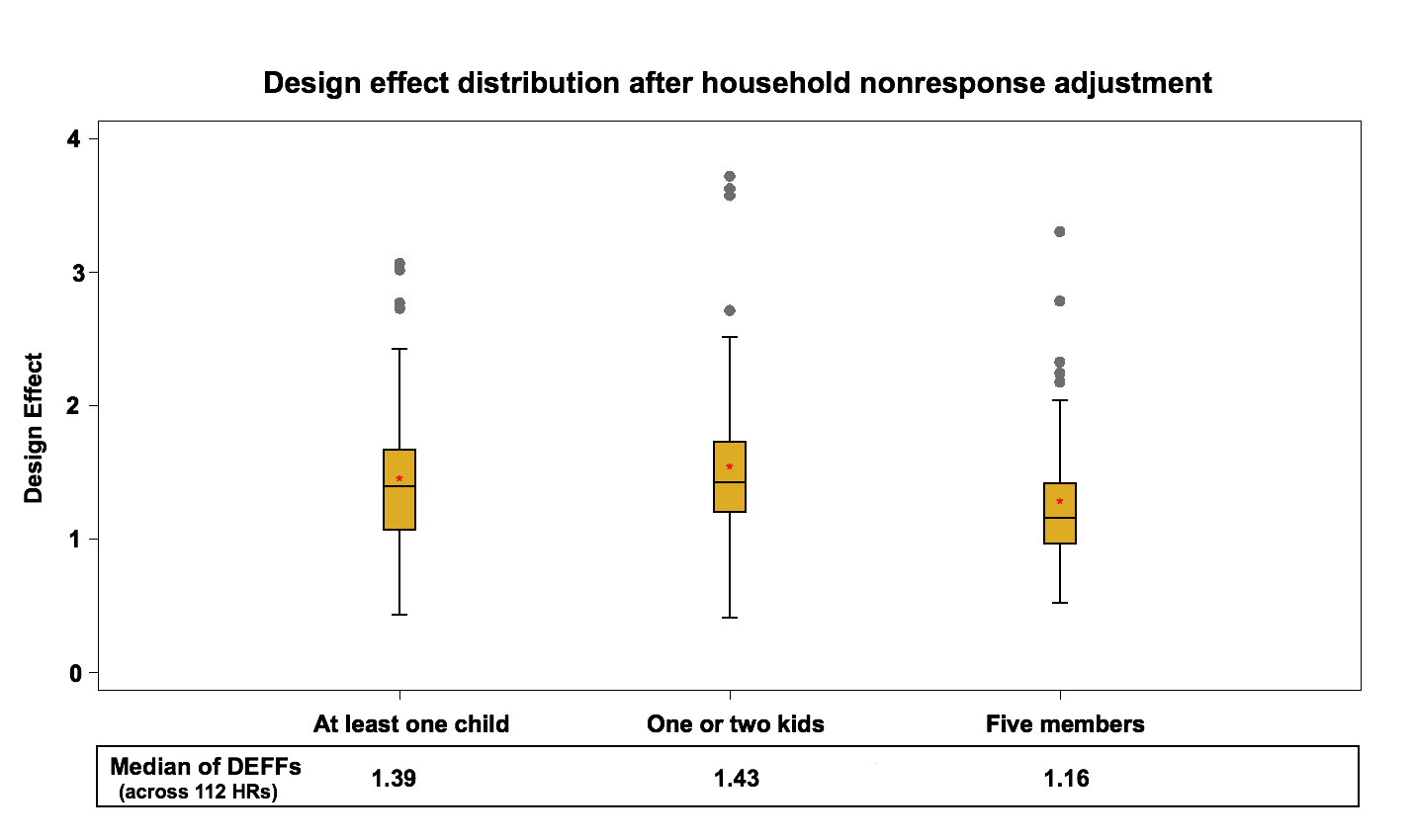
Figure 4: Design effect distribution (across 112 HRs) after the Household nonresponse adjustment in the area frame

Design effects go up slightly for both frames compared to the results of the previous step. The median design effect at the HR level varies between 1.2 and 1.4 for the area frame and between 1.1 and 1.2 for the telephone frame. This increase represents an average 8% increase on the area frame and 12% increase on the telephone frame.

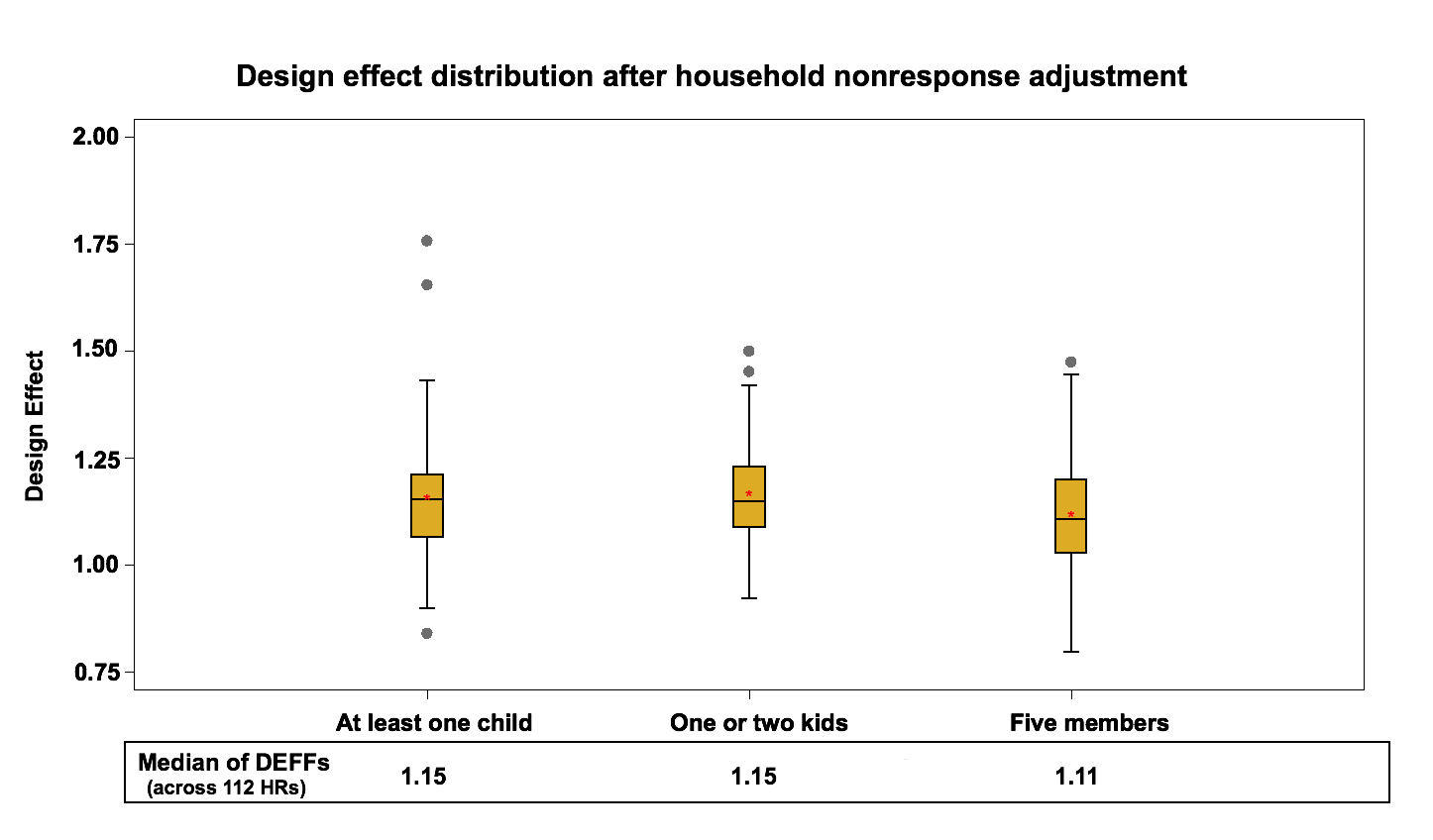
Figure 5: Design effect distribution (across 112 HRs) after the Household nonresponse adjustment in the telephone frame

This rise is expected since the nonresponse adjustment increases the variability of weights and therefore the variance of estimates in favor of reducing potential nonresponse bias. Also, the differences between the rises seen with the nonresponse adjustment on the two frames might be explained partly by the fact that there is more nonresponse on the telephone frame. In general, personal interviews have higher response rate comparing to the telephone interviews since the personal interviewers can make direct observation and generally do a better job of converting refusals.

4.3 Integration (Step I₁)

The third stage of interest for the study is the impact of the integration adjustment. At this step, the two frames are merged and the design effects of the variables after the integration- I1 adjustment are calculated.

The current integration approach takes into account the portion of the population covered by both frames which is a result of the under-coverage of the telephone frame. Those households without a landline or without a listed telephone number are not covered by the telephone list frame. Not taking this into account could cause a bias if the households not covered by the telephone frame have different characteristics than the ones covered. To take the under-coverage into consideration, the CCHS integrates only the sampled households that are common to both frames. The weights of the households that are only covered by the area frame (households without landline or without listed phone numbers) remain unchanged. This allows these households to represent other similar households in the population. For the common portion, the integration process applies a contribution factor to each frame. An adjustment factor α between 0 and 1 is applied to the weights; the weights of the area frame units that have telephone are multiplied by α and the weights of the telephone frame units are multiplied by 1-α. The term α represents the overall sample size contribution of the area frame to the common portion. A composite estimator for a total thus takes the form:

   

Where  represents the estimate, and  denote the area frame sample and the sample from the telephone frame, respectively. The subscript  indicates the common portion of both frames and  represents the portion of the area frame not covered by the list frame.

The term  has been fixed to 0.4 since 2008 for all domains which represent the overall sample size contribution of the area frame to the common portion in CCHS 2008. The reason of using a fixed  for all HRs and throughout time was to improve coherence and comparability between estimates over the domains and over time.  For more information, refer to Wilder and Thomas (2010). Figure 6 presents the design effect distribution at the HR level after Integration.

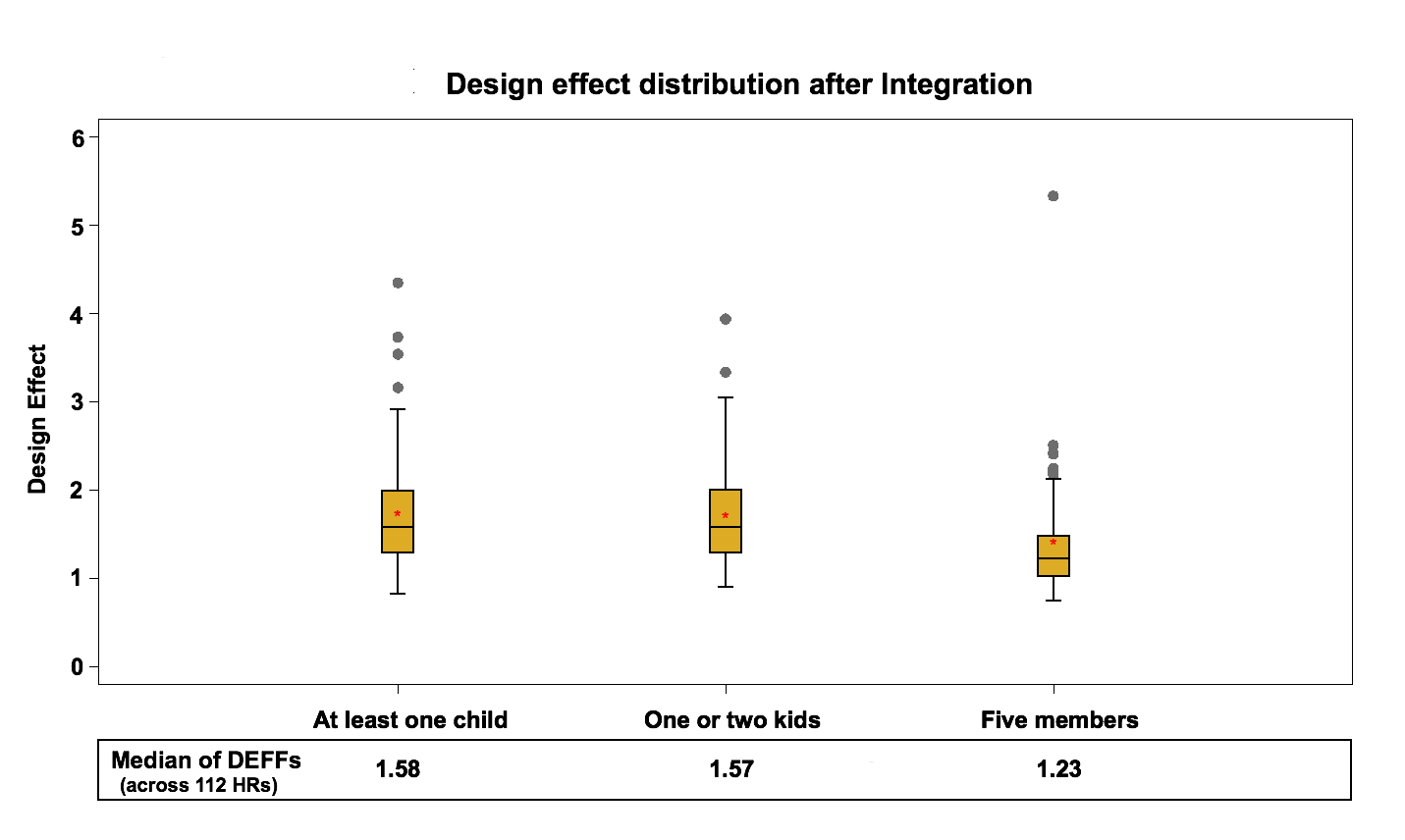
Figure 6: Design effect distribution (across 112 HRs) after Integration

There is an overall jump in design effects after joining the two frames, but a one-to-one comparison between design effects before and after integration is not possible since the two frames are combined. The median design effect within the health regions was between 1.2 and 1.4 for the area frame and between 1.1 and 1.2 for the telephone frame before integration. This amount increased to around 1.2 to 1.6 after integration for the combined sample. The increase can be explained by the fact that the integration adjustment adds a lot of variability to the weights. Only some units are adjusted and their weights are effectively halved. Also, there is the effect of using a fixed integration factor for coherence reasons rather than one based on efficiency of the estimator. A more efficient calculation of α would result in less impact on the variance.

4.4 The Person-Level Weight (Step I₂)

The fourth stage to be studied is the derivation of the person-level weight. At this stage, the concept of the variables examined in the study is changed since the statistical unit has now become the person rather than the household. The same concepts are preserved but estimates will now reflect characteristics in terms of people instead of households. These are:

• People living in households with at least one child (less than 12 years old)
• People living in households with one or two kids (less than 6 years old)
• People living in households with five members

At this step, the household-level weights are adjusted using the inverse of the person-level selection probabilities to calculate person-level weights. The person-level selection in the CCHS is done with unequal probabilities of selection based on the household size and the age of the household members.  For more information on the person-level selection probabilities, refer to the CCHS user guide, Statistics Canada (2011). Figure 7 presents the design effect distribution at the HR level after the creation of the person-level weight.

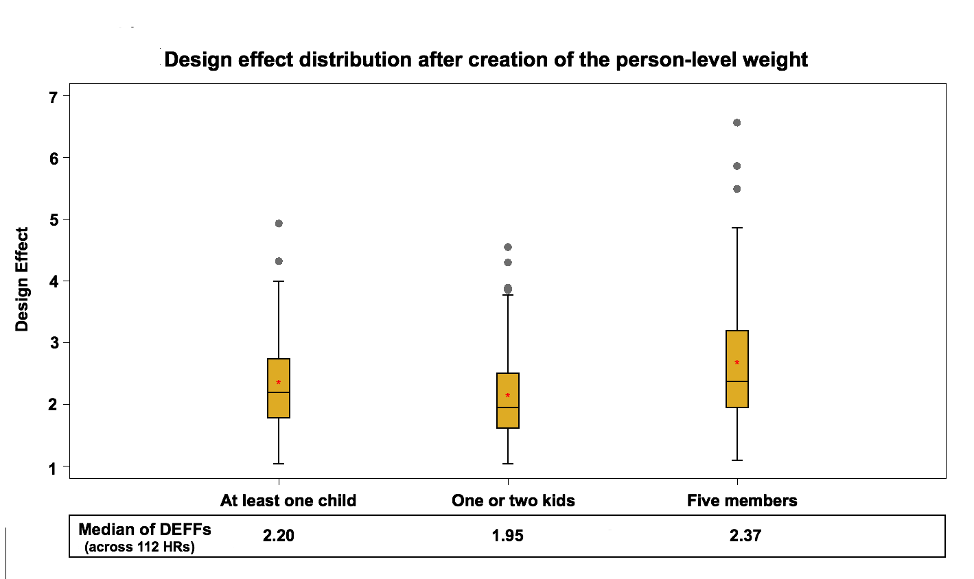
Figure 7: Design effect distribution (across 112 HRs) after creation of the person-level weight

The median of the design effect within health regions varies between 1.9 and 2.4. On average this is a 55% increase compared to the design effect calculated with the integrated household weight. This rise in the design effect is mainly due to the unequal probability of selection used by the CCHS. The person-level selection adjustment can be as low as 1 and as high as 20 in some cases. This design is quite different from what would have been observed with an SRS. One other reason for the increase in the design effect could be related to the change in variable concepts from household to person level. Estimates reflect the characteristics in terms of people instead of households.

4.5 Person-level nonresponse (step I₃)

The next step of the weighting adjustments to examine is the person-level nonresponse adjustment. As mentioned earlier, the CCHS interview has two parts: first the interviewer completes the list of the household’s members and then one person is selected for the interview. It is possible that the household roster is obtained (household response) but the selected person refuses to be interviewed or cannot be reached for some reasons. This causes person-level nonresponse. Among the responding households in 2010, 71315 individuals (one per household) were selected to participate to the survey, out of which a response was obtained for 63191 individuals, resulting in an overall person-level non-response rate of 11.4%.

The same treatment we used in household nonresponse is used at this stage where response homogeneity groups are created at the provincial level based on a logistic regression score function.

After creating response homogeneity groups, the following adjustment factor is calculated within each group:

 

   

The weights after step I₂ are multiplied by this factor to create the weights I₃. Figure 8 presents the design effect distribution for variables of interest at the HR level, after the person-level nonresponse adjustment.

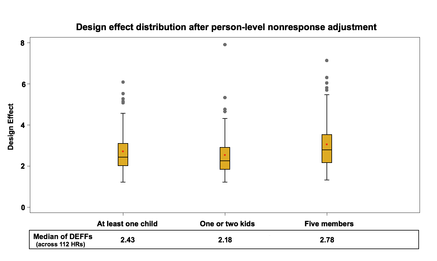
Figure 8: Design effect distribution (across 112 HRs) after person-level nonresponse adjustment

The median design effect at the health region level fluctuates between 2.2 and 2.8 while the median of the design effect in the previous step was between 1.9 and 2.4. This rise is expected and represents an average 9% increase. This is similar in nature to the household nonresponse adjustment. The nonresponse adjustment increases the variability of the weights, which leads to higher variance estimates in favor of reducing potential nonresponse bias.

At this level, the maximum design effect over the health region estimates can be as large as 7.91. This is due to the presence of extreme weights which are later adjusted by Winsorization (next step).

4.6 Winsorization (step I₄)

The sixth stage to be examined is Winsorization, which in the context of survey weighting consists in adjusting downward extreme weight values (Cox et al., 2011). Indeed, several steps of the weighting process may cause some units to end up with extreme weights, which will lead to the production of higher variance estimates. The winsorization can be seen as a correction measure reducing variance estimates at the cost of potentially introducing a small bias. Figure 9 presents the design effect distribution for after Winsorization.

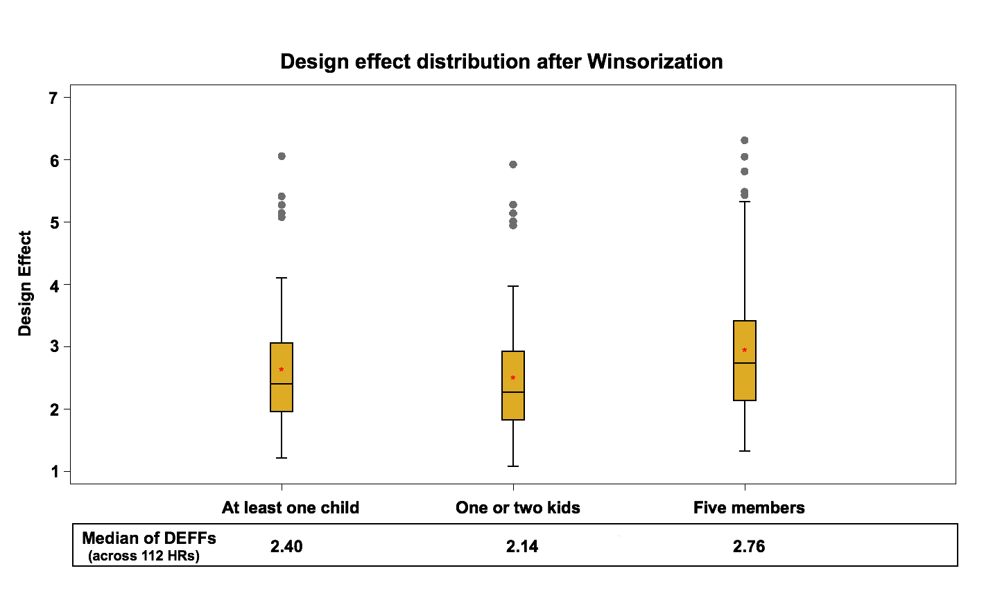
Figure 9: Design effect distribution (across 112 HRs) after Winsorization

After the winsorization step, the median design effect varies between 2.1 and 2.8. Comparing this with the results of the previous step, it can be concluded that winsorization does not have a significant effect on the median of the design effect mainly because very few units are winsorized. It does deflate the extreme values that were observed for some domains in the previous step which is the goal of this process.

4.7 Calibration (Step I₅)

The last step to study is calibration. This adjustment is done to make sure that the sum of the final weights corresponds to the population estimates defined at the HR level for each of the 10 age-sex groups. The five age groups are 12-19, 20-29, 30-44, 45-64 and 65+, for both males and females. At the same time, weights are adjusted to ensure that each collection period is equally represented in the population. Calibration is done using CALMAR (Sautory, 2003) with the most up to date population counts and the most up to date geographic boundaries. Figure 10 demonstrates the design effect distribution for variables of interest at the HR level, after the calibration adjustment.

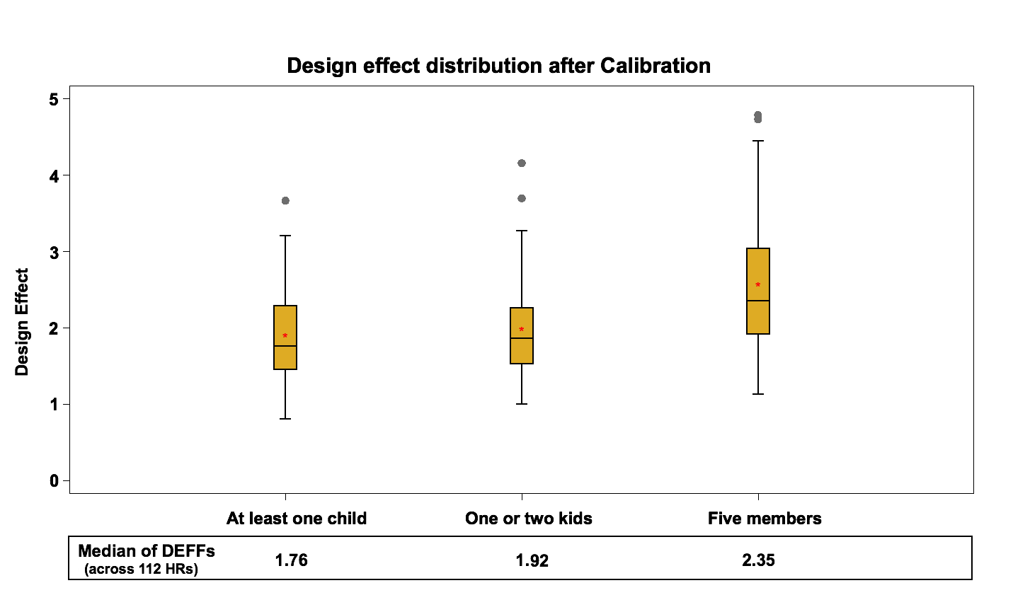
Figure 10: Design effect distribution (across 112 HRs) after Calibration

Based on past experiences with household surveys using similar common practices for calibration, the results on the design effects were as expected; this step significantly decreases the design effect by 14% on average for the 3 variables. The median of the design effect after calibration is about 1.8 to 2.4, compared to 2.1 to 2.8 at the previous step.

4.8 Summary

This section provides a graphical summary of the weighting adjustments’ impacts on the design effect for each variable at the HR level. For each variable the estimates of design effect are computed in 112 HRs. The median of these values (design effects) are presented in the following chart.

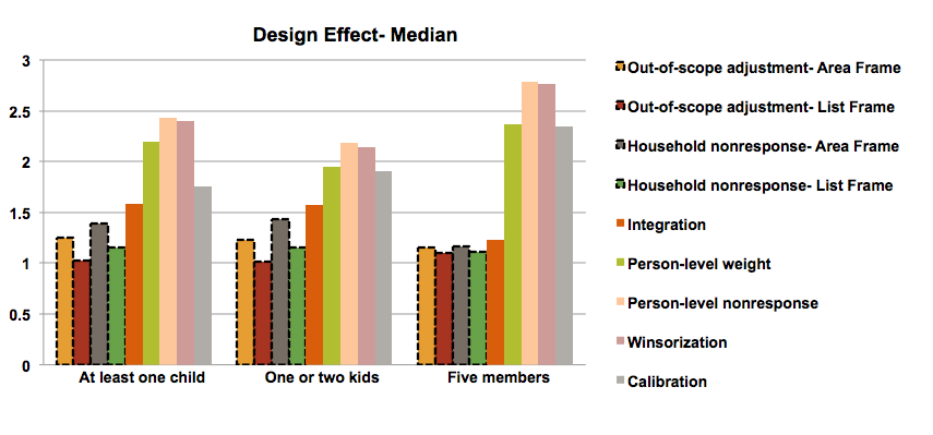
Figure 11: Median of design effects at the health region level

The first four bars (dashed outlined) represent the design effects of step 1 and step 2 for the area frame and the list frame separately (before integration) and the other bars show the design effects after integration (combined frame). The chart shows clearly that the person-level-weight and the nonresponse adjustments have the most negative impact on the design effect while calibration and winsorization decrease the design effect. The integration step has also a negative impact that is non-negligible.

The trend of the design effects throughout the weighting process is similar for all variables. However, we can notice some differences for the variable “household with five members” compared to the others. This is most likely due to how the design interacts with the variable of interest. Households with many members have different landline rates than those with fewer members. Also the person-level adjustment will have a larger impact on these types of households. This is also the variable with the lowest prevalence rate and large weights can have a greater impact on the variance and the design effects in this situation.

4.9  The role of the bootstrap method

The bootstrap method is an important part of this study, as design effects of different steps of weighting process are all derived from the bootstrap estimate of variances under the CCHS design. As mentioned earlier the Rao, Wu and Yue bootstrap method was used to estimate the design effects, and the number of bootstrap replicates was set to 500.

A key question would be how the Rao, Wu and Yue bootstrap method and number of replicates affect the results of this study. Mach et al. (2007) and Girard (2009) studied the Rao, Wu and Yue bootstrap method under different scenarios including different sampling method and nonresponse adjustment. In particular, Girard (2009) showed that even though the Rao-Wu bootstrap method considers the nonresponse mechanism as a deterministic process and does not fully capture the variance due to nonresponse, it provides reasonable estimates when the sampling fraction is small. Conceivably, the effect of the post-stratification and calibration on the estimate of variances would be ignorable if the number of the post-strata is not too large. Regarding the number of bootstrap replicates (BR), most of the literature suggests choosing sufficiently large number (Pattengale et al., 2010). We performed a simulation study and examined how the estimates of design effect vary using different number of replicates.

Figure 12 presents the design effect after calibration adjustment across 112 health regions with different number of bootstrap replicates for one of the variables of interest, household with one or two kids.

Figure 12:  Design effect across 112 HRs with different number of bootstrap replicates

Even though the overall display of design effect across 112 health regions does not change much and the median of the design effects fluctuates slightly, evaluating the design effect estimates for each health region shows that increasing the number of bootstrap replicates affects the estimates of design effect noticeably. In particular, the estimates of design effect for each health region vary 6% in average as the number of bootstrap replicates increases from 500 to 5000.

To address this issue, we estimated the design effect at different steps of weighting process for each health region, using different number of bootstrap replicates ranging from 500 to 5000. Comparing the estimates of design effect for each health region suggests that the estimates of design effect are not stable as the number of bootstrap replicates changes. For instance, Figure 13 shows the changes of design effect estimates for one of the health regions, HR 3565, after integration, person-level weigh, person-level nonresponse, winsorization and calibration adjustments.

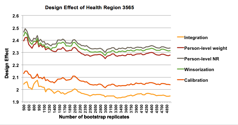
Figure 13: Design effect of Health Region 3565 with different number of bootstrap replicates

The fact that estimates of design effects are unsteady for different number of bootstrap replications does not contradict the results presented in previous sections, as the impact of the different steps of weighting adjustment on the design effect is still detectable. In other words, the instability of design effect does not invalidate the results of this study and we can still conclude that nonresponse adjustment has the most negative impact on the design effect and calibration and winsorization decrease the design effect.

5. Conclusion

In this paper, we empirically examined the effect of different steps of the weighting process on the efficiency of the Canadian Community Health Survey design, and showed which of the survey steps cause more variability in the estimates and cause the estimates to be less efficient compared to a simple random sample. The comparison results suggest that using unequal person-selection probabilities and the nonresponse adjustment considerably increase the variability of design. Similarly, using multiple frames under current integration method with fixed α has a negative effect on the design effect. On the other hand, winsorization and calibration using population counts decrease the design effect and improve the precision of the estimates. An interesting observation in the results is the design effects at the person level for variables with small prevalence are higher, especially when large weights are assigned to units that have the characteristic. Considering the above points, using only one frame which consists of a list of individuals instead of a list of dwellings would lower the design effect and reduce the variation. While results discussed here are valid in the frame work of CCHS they may be helpful for other multi-stage household surveys with similar complexities.

References

1. Béland, Y., Dale, V., Dufour, J., & Hamel, M. (2005). The Canadian Community Health Survey: Building on the Success from the Past. In Proceedings of the American Statistical Association Joint Statistical Meetings, Section on Survey Research Methods. Minneapolis: American Statistical Association.
2. Cox, B. G., Binder, D. A., Chinnappa, B. N., Christianson, A., Colledge, M. J., & Kott, P. S. (Eds.). (2011). Business survey methods (Vol. 214). John Wiley & Sons.
3. Gabler, S., Haeder, S., & Lahiri, P. (1999). A model Based Justification of Kish’s Formula for Design Effects for Weighting and Clustering. Survey Methodology, 25, pp. 105-106.
4. Girard, C. (2009). The Rao-Wu rescaling bootstrap: from theory to practice. In Proceedings of the Federal Committee on Statistical Methodology Research Conference, (pp. 2-4).Washington, DC: Federal Committee on Statistical Methodology.
5. Kalton, G., Brick J. M., & Lê, T. (2005). Chapter IV: Estimating Components of design effects for use in sample design. Household Surveys in Developing and Transition Countries. United Nations Publications.
6. Kish, L. (1965). Survey Sampling.  New York: John Wiley & Sons.
7. Kish, L. (1987). Weighting in Deft². The survey statistician, pp. 26-30.
8. Kish, L. (1992). Weighting for unequal P_i. Journal of Official Statistics, 8, pp. 183-200.
9. Lê, T., Brick J. M., & Kalton G. (2002). Decomposing Design Effects. In Proceedings of the American Statistical Association Joint Statistical Meetings, Section on Survey Research Methods. New York: American Statistical Association.
10. Mach, L., Saïdi, A. & Pettapiece, R. (2007). Study of the Properties of the Rao-Wu bootstrap variance estimator: What happens when assumptions do not hold?. In Proceedings of the Survey Methods Section, SSC Annual Meeting. St. John’s: Statistical Society of Canada.
11. Lehtonen, R., & Pahkinen, E. (2004). Practical Methods for Design and Analysis of Complex Surveys. Chichester: John Wiley & Sons.
12. Park, I., Winglee, M., Clark, J., Rust, K., Sedlak, A., & Morganstein D. (2003). Design Effect and Survey Planning. In Proceedings of the American Statistical Association Joint Statistical Meetings, Section on Survey Research Methods. San Francisco: American Statistical Association.
13. Pattengale, N. D., Alipour, M., Bininda-Emonds, O. R., Moret, B. M., & Stamatakis, A. (2010). How many bootstrap replicates are necessary?. Journal of Computational Biology, 17(3), 337-354.
14. Rao, J.N.K., Wu., C.J.F., &  Yue, K. (1992). Some Recent Work on Resampling Methods for Complex Surveys. Survey Methodology, 18, 209-217.
15. Sarafin, C., Simard, M. & Thomas, S. (2007). A Review of the Weighting Strategy for the Canadian Community Health Survey. In Proceedings of the Survey Methods Section, SSC Annual Meeting. St. John’s: Statistical Society of Canada.
16. Särndal, C. E., Swensson, B., & Wretman, J. (1992). Model Assisted Survey Sampling. New York: Springer.
17. Sautory, O. (2003) CALMAR 2: A New Version of the CALMAR Calibration Adjustment Program. In Proceedings of Statistics Canada International Symposium, Challenges in survey taking for the next decade. Ottawa: Statistics Canada.
18. Statistics Canada (2011). Canadian Community Health Survey (CCHS) Annual component; User guide, 2010 and 2009-2010 Microdata files. Statistics Canada.
19. Statistics Canada (2005), User Guide (BOOTVAR 3.1 ­ SAS Version), Statistics Canada, Available from: http://www.statcan.gc.ca/rdc-cdr/bootvar_sas-eng.htm
20. Wilder, K., & Thomas, S. (2010). Dual frame Weighting and Estimation Challenges for the Canadian Community Health Survey. In Proceedings of Statistics Canada International Symposium, Social Statistics: The Interplay among Censuses, Surveys and Administrative Data. Ottawa: Statistics Canada.
21. Yeo, D., Mantel, H., & Liu, T. P. (1999). Bootstrap variance estimation for the national population health survey. In Proceedings of the American Statistical Association Joint Statistical Meetings, Section on Survey Research Methods. Baltimore: American Statistical Association.