

Finding Respondents in the Forest: A Comparison of Logistic Regression and Random Forest Models for Response Propensity Weighting and Stratification
Special issue
Buskirk, T. D. & Kolenikov S. (2015), Finding Respondents in the Forest: A Comparison of Logistic Regression and Random Forest Models for Response Propensity Weighting and Stratification. Survey Insights: Methods from the Field, Weighting: Practical Issues and ‘How to’ Approach. Retrieved from https://surveyinsights.org/?p=5108
© the authors 2015. This work is licensed under a Creative Commons Attribution 4.0 International License (CC BY 4.0) 
Abstract
Survey response rates for modern surveys using many different modes are trending downward leaving the potential for nonresponse biases in estimates derived from using only the respondents. The reasons for nonresponse may be complex functions of known auxiliary variables or unknown latent variables not measured by practitioners. The degree to which the propensity to respond is associated with survey outcomes casts light on the overall potential for nonresponse biases for estimates of means and totals. The most common method for nonresponse adjustments to compensate for the potential bias in estimates has been logistic and probit regression models. However, for more complex nonresponse mechanisms that may be nonlinear or involve many interaction effects, these methods may fail to converge and thus fail to generate nonresponse adjustments for the sampling weights. In this paper we compare these traditional techniques to a relatively new data mining technique- random forests – under a simple and complex nonresponse propensity population model using both direct and propensity stratification nonresponse adjustments. Random forests appear to offer marginal improvements for the complex response model over logistic regression in direct propensity adjustment, but have some surprising results for propensity stratification across both response models.
Keywords
Logistic Regression, Nonresponse, Random Forests, Stratification, Survey Response Propensity Adjustments, weighting
Acknowledgement
We would like to thank our families and companies for their support of this work. We would also like to thank the reviewers for their thoughtful remarks that have helped improve the paper immensely.
Copyright
© the authors 2015. This work is licensed under a Creative Commons Attribution 4.0 International License (CC BY 4.0)
1 Introduction
Nonresponse is a common problem that impacts the validity of survey estimates. If respondents are different from non-respondents on important survey measures, analyses based only on respondents run the risk of nonresponse biases. To correct for the issue, various nonresponse adjustments can be made to the survey data ranging from simple nonresponse adjustment cell methods to more advanced nonresponse propensity adjustments (Kalton and Flores-Cervantes, 2003). The current research literature has provided a growing number of examples of models predicting survey response a priori survey administration and using estimated propensities to tailor survey design protocols (Buskirk, et al., 2013, Peytchev et al., 2010, Link and Burks, 2013 and Wagner, 2013 among others), but traditionally, response propensity models have been used as the basis for computing weighting adjustments to reduce the impact of nonresponse (Brick, 2013). In most typical applications of nonresponse adjustment, a model predicting the binary unit response outcome is fit using a set of variables available from the sample for both respondents and non-respondents. Unlike the weighting class adjustment methods which are typically restricted to categorical variables, and a limited number of them at that, response propensity models attempt to “balance” respondents and nonrespondents using a single propensity score that is a function of a host of both continuous and categorical predictors (Kalton and Flores-Cervantes, 2003). In this sense, nonresponse adjustments based on the propensity scores extend the weighting class method by allowing for the inclusion of many predictors and their interactions (Chen et al., 2012). The utility of this adjustment method relies on properly specifying and estimating the response propensity model – one that estimates well the corresponding, true propensity to respond to the survey invitation (Chen et al., 2012) – as well as on choosing predictors that are also associated with the survey outcomes of interest (Little and Vartivarian, 2005 and Brick, 2013). In cross-sectional surveys, predictor variables are typically frame data, survey paradata (Kreuter, 2013), interviewer observations or contact records (Wagner, 2013) or other variables that can be appended to the frames (Burks and Buskirk, 2012). In longitudinal surveys or repeated panel surveys, data from previous waves can also be used as covariates (Peytchev et al. 2010 and Meekins and Sangster, 2004).
Once the models are estimated, response propensities can be derived and then applied as the basis of survey nonresponse adjustments using one of two broad techniques (Brick, 2013) – direct adjustment or adjustment based on propensity stratification. The direct approach, or response propensity weighting (RPW), applies a nonresponse adjustment factor to the base weights of respondents which is computed as the inverse of the estimated response propensity (Bethlehem et al., 2011, Valliant et al., 2013 and Chen et al., 2012). This approach can produce highly variable weights especially if the propensity models produce predicted probabilities close to zero (Little, 1986; Brick, 2013). In contrast, the propensity stratification weighting (PSW) approach borrows from the standard treatment effect estimation literature and combines cases with similar values of predicted response propensities to form nonresponse adjustment cells or strata (Little, 1986). The nonresponse weighting adjustment factor is then usually defined in one of three ways: (a) the inverse of the average response propensity in a given cell; (b) the ratio of the sum of the input weights of all cases in the cell to the sum of the input weights of the respondents in the cell; or (c) the inverse of the unweighted response rates within each cell (Bethlehem et al., 2011 and Valliant et al., 2013). While there is limited guidance or research into the optimal number of such nonresponse adjustment cells, both Cochran (1968) and Rosenbaum and Rubin (1983) have suggested using 5 in practice. Several different approaches have been offered to form these nonresponse cells (also referred to as endogenous strata in the treatment effect estimation literature) including: using quintiles or deciles of the distribution of estimated response propensities, or using iterative procedures for determining optimal number and nature of the adjustment cells based on balancing auxiliary variables across survey response status (Imbens and Rubin, 2010). The simplest approach that incorporates Cochran’s suggestion as well as the theory for making the response propensities within each stratum as alike as possible is to use classes defined by equal length (see Bethlehem et al., 2011 for an example). For the comparisons presented here, we adopt this approach and use 5 classes of equal length to form the propensity strata.
Response propensities are often modeled using logistic or probit regression (Chen et al., 2012). However, newer techniques for classification and modeling have also been explored as methods for generating response propensities including local polynomial regression (Da Silva and Opsomer, 2009) and classification and regression trees (Phipps and Toth, 2012 and Valiiant et al., 2013). To date the literature on the use of other nonparametric machine learning techniques such as random forests (Breiman, 2001) has been limited. Random forests are an example of a nonparametric “ensemble” tree-based method because they generate estimates by combining the results of several classification or regression trees rather than using the results of a single tree. By aggregating estimates across many trees, random forests tend to generate more stable estimates compared to those generated from a single tree (Brieman, 2001). Buskirk et al. (2013) illustrated the use of random forests for predicting survey response in future surveys and discuss how to use the derived propensities as part of a tailored survey design. McCarthy et al. (2009) provided an overview of the use of similar data mining techniques in producing overall official statistics. In the current literature, however, there has been limited research comparing the direct use of random forests to logistic regression models for nonresponse adjustments based on estimated response propensity models.
Random forests and related nonparametric approaches relax the assumptions regarding the form of the propensity models and adapt to the size and complexity of the underlying data at hand (Margineantu and Dietterich, 2002). While the sample size is not usually the primary determinant of the final set of candidate predictors to be considered in a logistic regression model estimating survey response, it can certainly influence it. For example, if there are not sufficient respondents for a given level of a candidate factor, response propensity models estimated using logistic regression may fail to converge because of quasi-complete separation (Alison, 2008). To avoid this issue, one possibility is to reduce the size of the final set of predictors by eliminating the variable in question from the model building process. While this approach avoids the convergence issue, it does introduce the possibility of bias from model misspecification. Convergence issues like this can be exacerbated if the model is to contain the interaction between two factors that are associated like age group and education level – two variables that are commonly related to survey response (Groves, 2006). The association between these two variables, for example, may lead the researcher to potentially include them only as main effects if there aren’t sufficient respondents who fall in the “young and advanced degree” cell, for example. Generally, this issue is less concerning for surveys with larger samples (e.g. national surveys). However, for surveys of smaller municipalities or geographies with smaller sample sizes, there is greater potential for model convergence issues related to sparseness, especially if there are many candidate predictors for modeling survey response. In contrast, random forests are well suited for both large data sets, with many respondents and predictors, as well as for the “large p, small n” situation (i.e. many candidate predictors, few respondents) and can also handle correlated predictors in estimation (Strobl et al., 2007) without the convergence concerns of logistic regression. By being more adaptable to both model form and complexity, random forests have the potential to improve the estimation of survey response over logistic regression, especially if the sample sizes are small relative to the number and type of predictors to be considered or if the response propensity behavior involves factor interactions or more complex terms that are not known by the researcher at the time the model is estimated (Mendez et al., 2008 and Ayer et al., 2010). The improvements in estimation of survey response should, in turn, result in improved survey estimates derived using sampling weights that have been adjusted using the more accurately estimated response propensities.
In this paper we compare the use of logistic regression and random forest models for generating nonresponse adjustments based on both response propensity weighting and propensity stratification weighting. This research extends the current literature by providing a direct comparison of a traditional method for response propensity estimation (i.e. logistic regression) to a relatively new nonparametric, data mining method (i.e. random forests). Each of these methods was used to estimate the likelihood of survey response based on a simple random sample selected from our target population – which is described in more detail in the next section. Respondents and nonrespondents in this sample were identified using survey response outcomes generated according to both a simple and complex response propensity model which we also describe in section two. In section three we present results evaluating the estimated propensities and the resulting weighting adjustments in terms of bias, design effects and mean squared errors for five survey outcomes using data from the target population. We close the paper in section four with conclusions and a discussion.
2 Data and Methods
2.1 Population and Sample Data
The population for this mini-simulation study comes from the 2012 US National Health Interview Survey (NHIS) which is the largest continuing face-to-face survey of the general residential population of the U.S. The annual NHIS sample size is about 35,000 households and 88,000 persons. Data collection includes a basic household questionnaire, a brief questionnaire completed for every member of the household and a more in depth questionnaire completed by one selected adult and one selected child per household. A more complete description of both the NHIS study and survey data is available at: http://www.cdc.gov/nchs/nhis.htm. Records from 26,785 persons aged 18+ with no missing values for education, income, health status and phone usage were extracted from the 2012 NHIS public-use survey data file and serve as our finite “target” population. The complete list of variables with non-missing values available for each adult in our target population is provided in Table 1. The NHIS was specifically chosen as the data source for this study because it is the only large-scale, publicly available data set in the U.S. that contains a phone usage which has been reported to be associated with several health related survey outcomes of interest (Blumberg et al., 2013) as well as to survey response(see Pew Research, 2012).
From our target population we selected a single simple random sample of 5,000 adults without replacement to serve as the sample for this study. The base sampling weight for each unit in our sample was computed simply as the inverse of the selection probability (i.e. wi=(5,000/26,575)-1 =5.357 for i=1,2,…,5000). The NHIS final sampling weights were not used in either sample selection or weighting as the intention was to isolate the effects of the different non-response adjustment methods applied to our fixed sample and evaluate the results in the context of a finite population with known population parameters. If we were taking weighted samples instead, we would not know if the discrepancies between the sample results and the population quantities are due to the adjustments that we study, or due to the informative sampling design.
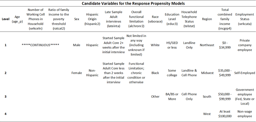
Table 1: Predictor variables used for generating survey response outcomes and subsequently estimating nonresponse propensity adjustments. Specific levels for the categorical predictors are also provided.
2.2 Creating Population Response Propensities and Survey Response Outcomes
In this paper we discuss, describe and use two types of propensities – generated and estimated. Generated (i.e., true, or population), response propensities are those that are assigned to each member of our target population using a response propensity model defined prior to selecting our sample and are intended to simulate survey response behavior. The generated response propensities are then used to create a binary survey response outcome for each adult in our sample in order to determine which sampled adults are survey “respondents” and which are “nonrespondents.” Applying either logistic regression or random forest methods to our sample with the survey response outcome as our dependent variable yields the estimated survey response propensities.
More specifically, for each member of the population, two different response propensities were generated using two different response propensity models that were based on a subset of the predictors provided in Table 1. The first of these models (referred to as RP Model 1) generated response propensities as a fairly straightforward function of three main effects including: age, sex and race and is depicted by equation A1.1 in Appendix 1. The second of these models (referred to as RP Model 2) generated survey response propensities as a more complex function of age, income, gender, education, cell phone ownership and interactions between income and education as well as interactions between cell phone ownership, age and gender as well as an interaction between landline ownership, age and gender. The equation used to generate these response propensities is displayed in equation A1.2 in Appendix 1. The specific coefficient values for each variable or term listed in equations A1.1 and A1.2 were selected to generate response propensities that would be as consistent with response patterns reported in the broader survey research literature as possible while at the same time balancing the overall range, mean and variability of the generated response propensities across the two response propensity models for the entire target population. The response propensities generated from RP Model 1 for the 5,000 sampled adults ranged from 0.155 to 0.825 with an average value of 0.530 and standard deviation of 0.148. Similarly, the response propensities generated from RP Model 2 for the 5,000 adults in our sample ranged from 0.150 to 0.893 with a mean of 0.532 and standard deviation of 0.148.
Each member in our sample was also assigned two survey response outcomes, independently, based on the response propensities generated from RP Model 1 and 2, respectively using an approach consistent with the stochastic framework described by Bethlehem (2002). More specifically, each adult in our sample was assigned a binary survey response outcome (referred to as Survey Response 1) by comparing the adult’s response propensity generated from RP Model 1 to a random UNIFORM(0,1) value. If the value of the uniform random draw for the sampled adult was less than or equal to the sampled adult’s response propensity generated from RP Model 1, then Survey Response 1 was set to 1; otherwise it was set to zero. The random draws from the uniform distribution were independently drawn for each adult. The process was repeated in its entirety to assign each sampled adult a value for the Survey Response 2 outcome variable (referred to as Survey Response 2) using the response propensities generated from RP Model 2 and a separate set of independent uniform random draws. We note that in our analyses, we used two versions of a single sample of 5,000 adults, rather than two separate samples. Essentially, the two variables, Survey Response 1 and 2, give two possible realizations of survey response under potentially different conditions (a simple and complex condition) for the same sample. The first realization based on Survey Response 1 resulted in 2,768 of the 5,000 sampled adults being identified as respondents; the second realization based on Survey Response 2 resulted in 2,682 of the 5,000 sampled adults being identified as respondents.
While we tried to generate response propensities for our target population using both a simple and complex model that are based on some of the collective results from the survey literature regarding survey response, the specific variables, or form in which they are included in our models, will certainly not be related to every possible survey outcome of interest, nor describe survey response behavior in every situation. So while the specific content and form of our models might not generalize to all applications, what does generalize is both the concept that the survey response mechanism is likely to be a complicated function of variables we have seen before and some that we have not and the strategy to use methods that can adapt to the complexity of these mechanisms using as many relevant variables as possible. Our primary intention is to begin to understand whether more contemporary methods, such as random forests, might be useful for the purposes of nonresponse adjustment and where traditional methods, such as logistic regression, may still be preferred. We describe these specific methods in greater detail in the next section.
2.3 Methods for Estimating Response Propensities
We employed different methods to estimate both of the binary survey response outcomes described in the previous section. The estimated response propensities obtained from each method using Survey Response 1 and Survey Response 2, as the outcome of interest reflect estimates of the response propensities generated from RP Model 1 and RP Model 2, respectively. More specifically, Survey Response 1 and 2 were estimated separately as a function of the predictor variables listed in Table 1 using four different methods including: (1) a main effects logistic regression model, (2) a stepwise logistic regression model, (3) a random forest classification model and (4) a random forest relative class frequency model. Each of these methods are described in the following subsections.
2.3.1 Logistic Regression Propensity Score Methods
For each of the two survey response outcomes we construct two different logistic regression models using the variables in Table 1. The first of these logistic regression models uses all of the variables in Table 1 and is referred to as the main effects logistic regression or more simple as ME Logistic Regression. Specifically, using our sample of 5,000 adults we estimate Survey Response 1 using all of the variables listed in Table 1, each of which is included in the model as a main effect. We apply this method again to estimate Survey Response 2. While complex interactions of predictor variables are likely predictive of survey nonresponse indicators, in general, main effects models seem to be the most commonly used among practitioners (Brick, 2013) so we include this method here as a baseline.
In addition to the main effects models, we computed separate stepwise logistic regression models for each of the two Survey Response outcomes. Each of the stepwise models was constructed in two stages. In the first stage, the respective full main effects regression model was reduced to a model with a smaller set of significant main effects by considering the removal or addition of each of the 13 possible variables in Table 1 in a stepwise fashion based on the Akaike Information Criterion (Akaike, 1974) model fit statistic. Unlike with other model fit criteria, both nested and non-nested models can be compared to one another using the AIC statistic. At the second stage deployed another stepwise logistic regression model that used the smaller set of significant predictors identified in stage 1. At the second stage the model also considered up to three-level interactions among the predictors as candidates for the final model and allowed for both the removal and addition of variables in a stepwise approach. We excluded the interaction of telephone status and the number of working cell phone numbers from consideration in the second stage stepwise model to avoid issues with convergence as the combination of these two variables devolves to only one level for adults who live in landline only households (i.e. number of working cell phones is constant at 0 for all landline only adults). Similar to the first stage, the stepwise procedure in the second stage also used the AIC measure of fit. Using the AIC (or some similar criterion) allowed the process of variable selection and inclusion to be automated with a clear identification of when the model building process should terminate. We refer to this method in its entirety as Step AIC logistic regression and note that the stepwise models were constructed separately using Survey Response 1 and 2 as the respective binary outcomes of interest. While we could have opted for a “best subset” approach over a step-wise approach, computing limitations made this option prohibitive. For example, the number of possible candidate models that would have been evaluated in such an approach using the 13 predictors allowing for up to three-level interactions exceeded 1 billion possible models. The stepwise approach has been used in elsewhere as well for comparing the utility of logistic regression models to classification trees (Phipps and Toth, 2012) for response propensity modeling.
2.3.2 Random Forest Propensity Score Methods
Before describing our alternative method of estimating response propensities, random forest, we need to introduce the building blocks of the forest – classification and regression trees (CART) (Breiman, Friedman and Stone, 1984). The difference between the classification and regression trees is only in the response being modeled, with regression trees used for continuous outcomes, and classification trees, for discrete outcomes (such as the binary survey response variables). A classification or a regression tree is a sequence of decisions to split the sample and to make a specific decision in each subset. Each decision is based on a single variable, so that one or more categories of a categorical variable are contrasted with other categories, and the values of a continuous variable below a certain cutoff point are contrasted with the values above the cutoff. The variables upon which splits are based, and the values/categories for those splits, are usually obtained by optimizing a goodness of fit criterion, such as root mean squared error for continuous outcomes, or misclassification error rates for categorical outcomes. The reason the method is referred to as a “tree” is because the decisions begin with the entire sample and branch forward in a recursive approach that can be visualized as a tree. Generally, classification trees are grown until the final nodes (called terminal nodes or leaves) either meet a minimum sample size requirement or are completely homogenous with respect to the outcome variable. Other decision rules affecting the complexity of the tree are discussed in greater detail by James et al. (2013), for example. An example tree for predicting Survey Response 1 using the variables listed in Table 1 is illustrated in Figure A3 of Appendix 3.
Developed by Breiman (2001), random forests are an ensemble-based method that generates estimates by combining the results from a collection (i.e. the ensemble) of classification or regression trees. More specifically, if the outcome of interest is continuous then a random forests model produces an estimate of the outcome by averaging the estimates derived from a series of regression trees. On the other hand, if the outcome is binary, a random forest generates an estimate defined as the category (e.g. either 0 or 1) that is predicted most often among a collection of classification trees. By combining results across an ensemble of trees, random forests avoid the over fitting tendency of any single tree and generate predictions with lower variance compared to those obtained from a single tree (James et al., 2013 and Breiman, 2001). Each tree in the forest is grown using an independently selected bootstrap subsample of the data set that is chosen with replacement and of the same size as the original dataset. Splitting in each of these trees occurs one node at a time and each tree in the forest is grown as large as possible.
The number of variables used for splitting each node is restricted to a random subsample of all possible predictor variables. The size of this subsample is the same for each node in each tree, is set by the user and is often referred to as “mtry.” The larger the value of this parameter, the more correlated trees in the forest become, reproducing the overfitting behavior that is typical for single trees, and thus resulting in higher overall prediction error rates. The smaller the value, the less correlated the individual trees are in the forest, resulting in lower overall prediction error rates; however, since the variables available for the splits are less likely to include the relevant ones, the trees have less predictive power. The most commonly used value for mtry that balances error with predictive power for classification is the square root of the total number of predictor variables available in the dataset rounded down to the nearest whole number and p/3 for regression with p predictors (Brieman, 2001). Apart from mtry, the other parameter of a random forest is the number of trees it has. In practical applications, this value is typically taken to be from 100 to 1000, with greater numbers providing more accurate and more stable estimates at the expense of computing time. For continuous outcomes, there is one additional parameter called node size which determines whether additional splitting on a node can occur or not. If the number of data points that fall in a node is larger than this threshold, additional splitting occurs; otherwise, the node becomes a terminal node in a given tree. The default value for node size for trees within forests applied to continuous outcomes is 5.
The overall prediction error of the random forest is generally a non-increasing, bounded function of the number of trees, meaning that after a certain number of trees, the additional reduction in error from adding additional trees to the forest becomes negligible (Brieman, 2001). However, it is also completely possible for a smaller forest to produce similar accuracy rates as a larger forest (Goldstein et al., 2011). While the value of mtry can impact the overall prediction accuracy of the forest, studies have indicated that the overall results tend to be fairly robust with similar performance being achieved across a fairly wide range of values (Pal, 2005). For continuous outcomes it has been shown in practice that prediction error rates can be reduced by using larger values of the node size parameter beyond the default (Segal, 2004).
We estimate propensity scores for our survey response outcomes using both a forest of classification trees as well as a forest of regression trees. First, we applied a random forest to each binary survey response outcome that consisted of a collection of classification trees. Under this approach the response propensity is estimated as the fraction of trees in the forest constructed without a given sampled adult that predict the adult to be a respondent. This estimate is considered to be “out of bag” since it is derived using trees in the forest that were grown without using the particular sampled adult (Breiman, 2001). This approach will be referred to as the random forest vote method. Next, we treated each binary survey response outcome as a continuous outcome and applied a random forest that consisted of a collection of regression trees and the estimated propensities are the relative frequency of respondents in the final node in which a given sampled adult falls averaged across all trees in the forest for which the given sampled adult is “out of bag” (Bostrom, 2007). We refer to this approach as the random forest relative frequency method (abbreviated random forest rel freq). Using either random forest method, roughly 32% of the trees from a forest were used to generate the propensity estimates based on the bootstrap sampling algorithm that is used by default for random forests (Breiman, 2001). In total we generate four random forests – one forest for each of the two methods applied to estimate each of the survey response outcomes.
Based on the results of preliminary tests we used 1,000 trees with mtry=3 for both the random forest vote method as well as the random forest rel freq method applied to estimate both of the survey response outcomes. Additionally, our preliminary tests for the node size parameter used for the relative frequency method indicated improvements in model fit by increasing the value from 5 to 20 for estimating both Survey Response 1 and 2. A more thorough discussion addressing the choices of these parameters is provided in Appendix 4. All calculations for this research were performed using R version 3.1.2 and the random forests were computed using the R package RandomForest.
2.4 Nonresponse Propensity Adjustments and Estimation of Survey Outcomes
As described elsewhere (Bethlehem et al., 2011 and Brick, 2013) nonresponse adjusted sampling weights are computed as the product of a propensity adjustment and the base weight. In some applications eligibility and multiplicity adjustments might have been applied to the base weights prior to applying the nonresponse adjustment (Buskirk and Kolenikov, 2013) but for our purposes we begin with the base weight that was previously described in section 2.1. To avoid mathematical irregularities in the weighting adjustments from cases with estimated propensities of 0 that were sometimes encountered, we based the nonresponse adjustments that we describe in this section on a small transformation of the estimated propensities that slightly shifted the estimates away from zero and one according to:
transformed estimated propensity = [(1000×estimated propensity+.5)/1001]
where 1000 represents the number of the trees used in the forest forests. This adjustment was similar in spirit to corrections for binomial data aimed at improving confidence interval coverage for proportions near zero or one (Agresti and Coull 1998), or to adjustments made to data that potentially contain zeroes prior to applying a logarithmic transformation in the general linear modeling context (Yamamura, 1999). For the remainder of the paper, all computations involving estimated propensities use these transformed values, so we will simply refer to them as the “estimated propensities” for the remainder of the paper.
Two versions of nonresponse adjusted weights were created from the estimated propensities obtained from each of the four methods for each of the two survey response outcomes. The first version, referred to as response or direct propensity weighting (RPW), applies a direct nonresponse adjustment factor to the base weight of each adult respondent in the sample computed as the inverse of the estimated propensity. The second version, referred to as propensity stratification weighting (PSW), applies an adjustment factor to the base weight of each adult respondent computed as the inverse of the weighted response rate for the propensity stratum containing the responding adult’s estimated propensity. Propensity strata were formed by dividing the range of the estimated propensity scores into 5 equal parts as illustrated by Bethlehem et al. (2011). We note that because the underlying base weights for each of the adults in our sample are equal (to 5.357, as described in Section 2.1), the use of weighted or unweighted response rates within each propensity stratum produces equivalent adjustment factors.
Final sampling weights were obtained by applying one additional scaling factor to the nonresponse adjusted weights equal to 26,785/SNBW where SNBW was the sum of the nonresponse adjusted base weights. This scaling factor was used to ensure that the sum of the final weights for any method or survey outcome summed to the size of our finite population. Our end goal was to evaluate biases in the weighted estimates and we used this scaling factor to put all of the final estimates on the same scale as the target population. While we could have introduced both trimming as well as additional post-stratification or calibration steps, we intentionally bypassed them in order to focus specifically on the impact of the nonresponse adjustments across the methods and to avoid any potential confounding that could have resulted from a combined nonresponse and trimming/calibration adjustment. This approach was consistent with the one adopted by Valliant and Dever (2011) who compared the impact of different propensity adjustment methods for weighting nonprobability surveys. Overall, this process produced a total of eight sets of final sampling weights per survey response outcome – one RPW set for each of the four methods and one PSW set for each of the four methods. The propensity strata used for computing the PSW weights were computed separately for each outcome and method. Similarly, the final scaling factor was also computed separately for each outcome, method and nonresponse adjustment type.
Survey estimates for one continuous and four binary population parameters are derived using these sets of final sampling weights: the mean Body Mass Index (BMI) for adults in our target population; proportions of adults in our target population who: have ever missed work due to illness in the past year; have seen a doctor/healthcare provider within the past year; are current smokers; and who have ever been told they have hypertension by a healthcare provider. The standard error calculations were performed using bootstrap replication (Rao and Wu, 1998) and are described in more detail in Appendix 5. In our target population, the hypertension and seen doctor outcomes were modestly positively correlated with the propensities generated by both RP Models 1 and 2 (0.30 and 0.20, respectively) and these two variables along with ever miss work were somewhat positively correlated with the response propensities generated by RP model 2 (0.06, 0.18 and 0.10, respectively). Ever missed work was moderately negatively correlated to the propensities generated from RP Model 1 (-0.16) while current smoker was somewhat negatively correlated with the propensities generated by both RP Models 1 and 2 (-0.09 and -0.14, respectively) in our population. By virtue of these correlations in our population, we would expect that estimates derived from only respondents could exhibit non-negligible response biases based on the stochastic view of nonresponse (Bethlehem 2002). Some evidence of this potential is illustrated in Table 2 below where it is apparent that the percentage of hypertension as well as the percentage who have seen a doctor are overestimated when using the unweighted sample of respondents defined by Survey Response 1. Similarly, the percentage of adults who are current smokers is underestimated and the percentage who have seen a doctor and overestimates the percentage who have seen a doctor when using the unweighted sample of respondents defined by Survey Response 2, for example.
We hypothesize that the logistic regression models, specifically the Step AIC version, will produce better estimates of the response propensities generated by RP Model 1 compared to the random forest models, since the form of RP Model 1 corresponds to a logistic regression model based on a subset of variables from Table 1. By virtue of the complex interaction effects included in RP Model 2, we also hypothesize that the random forest models will produce more accurate estimates of the response propensities generated by by RP Model 2. Bostrom (2007) reported that probability estimating trees for estimating propensities, which essentially use the relative frequency method with predictions derived using the entire forest rather than just the trees for which a case is OOB, have better results for generating propensity estimates compared to the forests based on classification trees (i.e. the vote method). In light of this research we expect that the random forest rel freq method will perform better than the voting model for the propensity adjustment methods and for estimating propensities.
|
Survey Outcome Variable |
Population Parameter (N=26,785) |
Mean/ Proportion from Full Sample (n=5,000) |
Mean/ Proportion from Respondents (RP model 1) (n=2,768) |
Mean/ Proportion from Nonrespondents (RP model 1) (n=2,232) |
Mean/ Proportion from Respondents (RP Model 2) (n=2,682) |
Mean/ Proportion from Nonrespondents (RP Model 2) (n=2,318) |
||
|
Body Mass Index |
27.918 |
27.997 (0.090) |
28.093 (0.120) |
27.877 (0.135) |
28.102 (0.123) |
27.874 (0.131) |
||
|
(27.858, 28.329) |
(27.860, 28.344) |
|||||||
|
Current Smoker |
0.196 |
0.197 (0.006) |
0.188 (0.007) |
0.207 (0.009) |
0.177 (0.007) |
0.220 (0.009) |
||
|
(0.173, 0.202) |
(0.162, 0.191) |
|||||||
|
Seen Doctor last year |
0.819 |
0.818 (0.006) |
0.837 (0.007) |
0.795 (0.009) |
0.833 (0.007) |
0.802 (0.008) |
||
|
(0.824, 0.851) |
(0.819, 0.847) |
|||||||
|
Ever miss work last year |
0.300 |
0.297 (0.006) |
0.273 (0.008) |
0.327 (0.010) |
0.315 (0.009) |
0.276 (0.009) |
||
|
(0.257, 0.290) |
(0.298, 0.333) |
|||||||
|
Ever told of Hypertension |
0.322 |
0.323 (0.007) |
0.358 (0.009) |
0.279 (0.009) |
0.332 (0.009) |
0.312 (0.010) |
||
|
(0.340, 0.376) |
(0.314, 0.349) |
|||||||
Note: There were 4 observations missing the ever miss work variable(3 nonrespondents and 1 respondent under RP Model 1 and 2 nonrespondents and 2 respondents under RP Model 2).
Table 2: Parameter values and estimates from the entire sample, as well as the sample of respondents and nonrespondents defined by both Survey Response 1 and 2. Standard errors are provided in parentheses next to the estimates and 95% confidence intervals derived using only the respondent samples (without any adjustments for nonresponse) are provided below the estimates in the respective columns.
3 Empirical Results
In this section we present the results separately by survey response outcome. Specifically, we first present and evaluate the estimated response propensities and final sampling weights and survey estimates obtained by applying each of the four methods to estimate Survey Response 1. We focus on comparisons across methods for the response propensities. For the final sampling weights as well as final survey estimates we make comparisons across the methods first for nonresponse adjusted weights using the RPW approach and second using the PSW approach. In the second half of this section, the corresponding results and comparisons are presented based on applying each of the four methods to estimate Survey Response 2.
3.1 Survey Response 1: Estimated Propensities
Overall descriptive statistics for the response propensities estimated from each of the four methods applied to Survey Response 1 are displayed in Table 3 and are based on the entire sample of 5,000 adults. Overall, the estimated propensities from the two logistic regression methods as well as the random forest rel freq method were similar. However, the random forest vote method produced estimated propensities with the broadest range and were the most variable. These methods exhibited nearly similar potential to differentiate respondents from nonrespondents (defined by Survey Response 1) based on the area under the receiver operating characteristic curve (AUC; Harrell 2010) (Table 3) but the logistic regression methods edged out the forest methods by a positive margin of about 0.045.
|
Method for estimating propensities for Survey Response 1 from RP Model 1(A1.1) |
Mean |
Std. Dev. |
Median |
IQR |
Min. |
Max. |
AUC |
|
|
ME Logistic Regression |
0.554 |
0.156 |
0.557 |
0.232 |
0.132 |
0.871 |
0.682 |
|
|
StepAIC Logistic Regression |
0.554 |
0.155 |
0.556 |
0.229 |
0.147 |
0.849 |
0.681 |
|
|
Random Forest Vote |
0.564 |
0.193 |
0.576 |
0.294 |
0.054 |
0.994 |
0.637 |
|
|
Random Forest Rel Freq |
0.553 |
0.150 |
0.568 |
0.233 |
0.130 |
0.911 |
0.658 |
|
|
Propensities Generated from RP Model 1 |
0.530 |
0.148 |
0.530 |
0.220 |
0.155 |
0.825 |
N/A |
|
Table 3: Summary statistics for the propensities estimated for Survey Response 1 for each of the four methods based on our sample of 5,000 adults.
The results of the StepAIC logistic regression method applied to estimate Survey Response 1 are given in Table A2.1 of Appendix 2. As can be seen there, the StepAIC logistic regression method identified the same main effects as specified in RP Model 1 (A1.1). The coefficients resulting from the StepAIC method are similar in both magnitude and sign to those used in RP Model 1 (A1.1) and consequently, the correlation observed between the propensities estimated using the StepAIC method and those generated from RP Model 1 was extremely high (0.997) as indicated in the diagonal of Table 4. A similarly high correlation was also observed between the propensities estimated using the ME logistic regression method and those generated by RP Model 1 (0.989). While still appreciably high, the same correlation for the random forest vote method was just under 0.80. Correlations between the estimated propensities for the four methods for Survey Response 1 are also provided in the LOWER triangle of Table 4. By virtue of the very high correlation measures provided, there was little differentiation between the propensities estimated from the two logistic regression methods as indicated by the very high linear correlation between them (r=0.992). Slightly lower correlation was observed between the propensities estimated using the two random forest methods, however (r=0.947).
|
ME Logistic |
StepAIC Logistic |
Random Forest Vote |
Random Forest Rel Freq |
|
|
ME Logistic |
1: 0.989; 2:0.857 |
0.987 |
0.722 |
0.807 |
|
StepAIC Logistic |
0.992 |
1: 0.997; 2:0.864 |
0.723 |
0.810 |
|
Random Forest Vote |
0.805 |
0.801 |
1: 0.799; 2:0.799 |
0.953 |
|
Random Forest Rel Freq |
0.909 |
0.907 |
0.947 |
1: 0.904; 2:0.895 |
Table 4. Correlation matrix for the estimated response propensities across the four methods from modeling Survey Response 1 (lower triangle) and from modeling Survey Responses 2 (upper triangle). The first value along the diagonal for each row represents the correlation between the response propensities estimated by the method in that row and those generated by RP Model 1. The second value listed in the diagonal for a given row represents the correlation between the propensities estimated by the method in that row and those generated under RP Model 2.
3.2 Survey Response 1: Final Sampling Weights and Survey Outcome Estimates
Summary statistics for the final sampling weights for the 2,768 respondents identified from Survey Response 1 for each of the four methods computed using the RPW and PSW approaches are presented in the left portion of Table 5A and 5B, respectively. We note that the means of the final sampling weights from each method under both the RPW and PSW approaches are all equal by virtue of the final adjustment made to each set of sampling weights to ensure that they sum to the size of our finite population. We will first focus on the weights and survey estimates obtained using the RPW approach for nonresponse weighting and then on the weights and survey estimates obtained using the PSW approach.
3.2.1 Final Sampling Weights from the RPW Approach and Resulting Survey Outcome Estimates
From the left panel of Table 5A we see that the summary measures for the two logistic regression methods and the random forest rel freq method are generally very similar. In line with the results presented in Section 3.1, the final sampling weights for the random forest vote method are the most variable and have the largest range. While large weights are not necessarily disadvantageous for producing final estimates, they do suggest a potential risk for producing estimates with higher variance. We examine this potential in the right panel of Table 5A which presents the estimates for the five survey outcomes of interest using the final sampling weights computed using the RPW approach for each of the four methods.
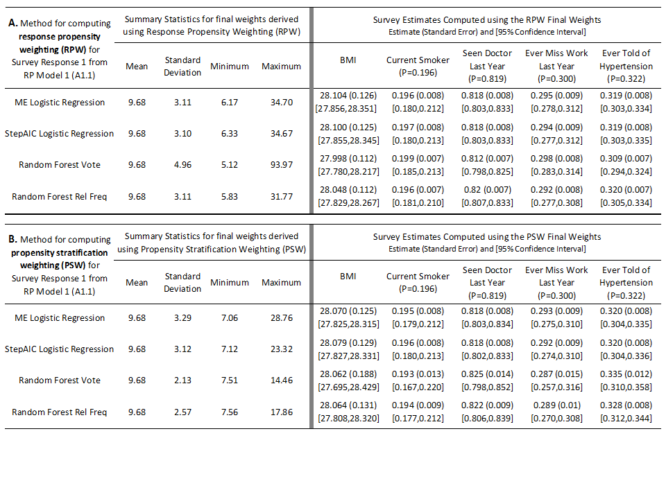
Table 5. Left Panels: Summary statistics for the final weights derived by applying response propensity weighting (top, A) and propensity stratification weighting (bottom, B) computed from each of the four methods for Survey Response 1 (A1.1). Right Panels: Final survey estimates computed using final weights derived by applying the response propensity weighting (top, A) and propensity stratification weighting (bottom, B) computed from each of the four methods for Survey Response 1 (A1.1). The standard errors based on bootstrap replication are given in parentheses and 95% confidence intervals are given in brackets below the estimates. The population parameter values for the key outcome variables are also provided under the variable names, for reference.
The final sampling weights from the two logistic regression methods produced similar estimates and standard errors for each of the five survey outcomes of interest. And while the random forest vote method produced the largest and most variable final sampling weights, the standard errors for each of the five survey estimates from this method are smaller than those produced using either of the logistic regression methods and equal to (up to three decimal places) those produced using the random forest rel freq method. There are also slight differences in the magnitude of the estimates across the methods for each survey outcome – the most notable difference being between the random forest vote method and the other three for the estimates of the proportion of adults ever told of hypertension and seen doctor in the past year. The 95% confidence intervals for each of the five survey outcomes for each of the four methods contain the actual parameter values for our finite population.
Putting together the estimated bias (difference between the weighted survey and the population parameter) and the standard errors for each of the five survey outcomes produces the mean squared errors (MSE) and design effects provided in Table 6A. The design effect estimates are squared DEFT statistics (Kish, 1965) and represent an estimate’s variance using the final sampling weights relative to the variance one would obtain using a simple random sample of the same size selected with replacement. From the table it is apparent that both random forest methods produce lower design effects for each of the five outcomes compared to either of the logistic regression methods. While the random forest vote method estimates were further away from the population parameters (higher estimated biases) for three of the five survey outcomes, overall the final survey estimates obtained from either the random forest vote or rel freq method had smaller estimated MSEs compared to those obtained from either of the logistic regression methods. This result is important to note – while we would have expected slightly higher biases from the random forest models by virtue of the worse fit between the estimated propensities and those generated by RP Model 1 discussed in the previous section, the overall error (bias and variance) from either of the random forest models seems lower compared to that from the logistic regression models. And while these errors were generally low across methods and survey outcomes, the MSEs for BMI and ever miss work percentage for estimates based on the random forest vote method were approximately half of those obtained from either of the logistic regression methods. Similarly, the MSEs for the estimates based on the random forest rel freq method for current smoker, seen doctor and hypertension rates were about 15 to 20 percent smaller than those estimated using either of the logistic regression methods.
|
A. Method for computing response propensity weighting (RPW) for Survey Response 1 from RP Model 1 |
Estimated Design Effects and Mean Squared Errors# for Survey Estimates Computed using the RPW Final Sampling Weights |
||||||
|
BMI |
Current Smoker |
Seen Doctor Last Year |
Ever Miss Work Last Year |
Ever Told of Hypertension |
|||
|
ME Logistic Regression |
1.110 |
1.196 |
1.106 |
1.020 |
0.799 |
||
|
50.37710 |
0.06811 |
0.06022 |
0.10522 |
0.07524 |
|||
|
StepAIC Logistic Regression |
1.090 |
1.235 |
1.121 |
1.078 |
0.845 |
||
|
48.81439 |
0.07064 |
0.06078 |
0.11530 |
0.07565 |
|||
|
Random Forest Vote |
0.892 |
0.904 |
0.874 |
0.816 |
0.726 |
||
|
18.94217 |
0.06095 |
0.10380 |
0.06589 |
0.22567 |
|||
|
Random Forest Rel Freq |
0.879 |
0.916 |
0.832 |
0.796 |
0.697 |
||
|
29.38921 |
0.05246 |
0.04483 |
0.12132 |
0.05927 |
|||
|
B. Method for computing response propensity weighting (PSW) for Survey Response 1 from RP Model 1 |
Estimated Design Effects and Mean Squared Errors# for Survey Estimates Computed using the PSW Final Sampling Weights |
||||||
|
BMI |
Current Smoker |
Seen Doctor Last Year |
Ever Miss Work Last Year |
Ever Told of Hypertension |
|||
|
ME Logistic Regression |
1.096 |
1.244 |
1.148 |
1.029 |
0.798 |
||
|
38.85368 |
0.07161 |
0.06214 |
0.13648 |
0.06730 |
|||
|
StepAIC Logistic Regression |
1.156 |
1.249 |
1.130 |
1.130 |
0.867 |
||
|
42.38303 |
0.07109 |
0.06269 |
0.14665 |
0.07191 |
|||
|
Random Forest Vote |
2.468 |
3.151 |
3.690 |
3.081 |
1.885 |
||
|
55.90062 |
0.18520 |
0.23242 |
0.40933 |
0.30239 |
|||
|
Random Forest Rel Freq |
1.203 |
1.397 |
1.406 |
1.280 |
0.853 |
||
|
38.51264 |
0.08357 |
0.08610 |
0.22087 |
0.10433 |
|||
Table 6. Design effects (top number in each cell) and Mean Squared Error estimates (bottom/bold number in each cell) for each of the five survey outcomes using the final sampling weights for each method based on response propensity weighting (top–A) and propensity stratification weighting (bottom–B) for Survey Response 1 (A1.1). # The MSEs presented in this table represent the actual MSE’s multiplied by a factor of 1,000 to illustrate differences.
3.2.2 Final Sampling Weights from the PSW Approach and Resulting Survey Outcome Estimates
The summary statistics for the final sampling weights using the PSW approach for nonresponse adjustment from each of the four methods applied to estimate Survey Response 1 appear to be fairly consistent for the two logistic regression models and the random forest rel freq method (Table 5B – left panel). For the PSW approach however, the random forest vote method final sampling weights appear to be the least variable and have the tightest range – a result that suggests that the number of respondents and nonrespondents in the lower and upper propensity strata, respectively, was greater than for any other method. This result could explain why the direction of the biases for the estimates obtained from the random forest vote method for the PSW approach are generally opposite of those of the RPW approach. The random forest vote method resulted in low estimated propensities for a number of respondents which in turn resulted in larger sampling weights using the RPW approach. However, because there were more of these respondents in the lowest propensity strata, their corresponding final sampling weight from the PSW approach would be much smaller. For example, the respondent who had the largest and most outlying sampling weight from the random forest vote method under the RWP approach and this weight was nearly double that from any other respondent. This adult also had the largest weight from the PSW approach, but this weight was only 14 compared to about 94 from the RPW approach. This respondent was a current smoker, had not seen a doctor, had missed work and was never told of hypertension. Given this profile, it is completely possible that the driver in the shifts in the estimates between the RPW and PSW approaches for the random forest method could be traced back to the large decrease in this respondent’s sampling weight combined with the fact that the sampling weights from the PSW approach had a much smaller range and were less disparate across respondents. The differences in the highest RPW and PSW weight across the other three methods were not as wide and the biases in the respective estimates seem generally consistent and in the same direction.
While the final sampling weights for the random forest vote method were more constrained, the standard error for the estimates obtained from this method were at least 50% larger than those obtained from any of the other methods. Moreover, estimates generated using the random forest vote method were nearly on par with the other methods for most variables except hypertension and seen doctor. For these outcomes, the random forest vote method estimates exhibited the largest amount of absolute bias compared to estimates from the other methods. And while the random forest vote method performed well with the RPW approach in terms of overall accuracy and MSE, the story is completely reversed for the PSW approach. From Table 6B we see that the overall design effects as well as the MSEs are larger for the random forest vote method compared to either of the logistic regression methods – in some cases between two and four times as large. The MSEs for the estimates obtained from the random forest rel freq method are only slightly larger than those obtained from either of the logistic regression for each one of the survey outcomes. And while the overall MSEs were generally small across all the methods and outcomes, the large difference between the accuracy of the random forest vote method compared to the other suggests that this method might not be practical or optimal to use with the PSW approach.
3.3 Survey Response 2: Estimated Response Propensities
Descriptive statistics for the response propensities estimated from each of the four methods applied to Survey Response 2 are displayed in Table 7 and are based on the entire sample of 5,000 adults. Generally, the results from the two logistic regression models are consistent and the random forest vote method exhibits the widest range of estimated propensities with the most variability. Our hypotheses regarding Survey Response 2 are partially supported by the correlations that are presented as the second entry along the diagonal in Table 3. There we see that the random forest methods had both the lowest (vote method, r=0.799) and highest (rel freq method, r=0.895) correlations between the estimated propensities and those generated using RP Model 2. The correlations between these quantities for the two logistic regression methods fell between these extremes. The final estimates produced using the StepAIC method for estimating Survey Response 2 are provided in Table A2.2 in Appendix 2. The coefficients from this model are not on the same scale as those listed in RP Model 2 (A1.2) and thus are not directly comparable. But one aspect of this model that is consistent with our hypothesis and merits mention is the relative lack of complexity in terms of higher order interactions – especially between income and education that are included in RP Model 2. However, despite these omissions in the estimated model (Table A2.2), the correlation between the estimated propensities and those generated from RP Model 2 for the StepAIC logistic regression method fall just under the correlation for the random forest rel freq method. The correlation measures in the upper triangle in Table 3 also indicate that the estimated propensities are not as highly correlated across the methods for Survey Response 2. There was also little variation between each method’s ability to differentiate between respondents and nonrespondents in the sample (as identified by Survey Response 2) as quantified by the AUC statistics in Table 7.
|
Method for computing response propensities for Survey Response 2 from RP Model 2 (A1.2) |
Mean |
Std. Dev. |
Median |
IQR |
Min. |
Max. |
AUC |
|
ME Logistic Regression |
0.536 |
0.142 |
0.528 |
0.225 |
0.213 |
0.839 |
0.664 |
|
StepAIC Logistic Regression |
0.536 |
0.142 |
0.526 |
0.220 |
0.211 |
0.827 |
0.662 |
|
Random Forest Vote |
0.540 |
0.200 |
0.549 |
0.281 |
0.008 |
0.992 |
0.646 |
|
Random Forest Rel Freq |
0.536 |
0.152 |
0.542 |
0.212 |
0.111 |
0.896 |
0.664 |
|
Propensities Generated from RP Model 2 |
0.532 |
0.148 |
0.529 |
0.212 |
0.150 |
0.893 |
N/A |
Table 7: Summary statistics for the propensities estimated for Survey Response 2 for each of the four methods based on our sample of 5,000 adults.
3.4 Survey Response 2: Final Sampling Weights and Survey Outcome Estimates
3.4.1 Final Sampling Weights from the RPW Approach and Resulting Survey Outcome Estimates
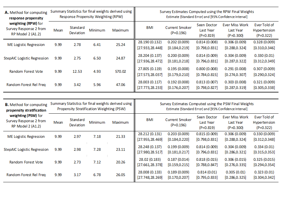
The final sampling weights derived using the RPW nonresponse adjustment approach from each of the four methods applied to estimating Survey Response 2 are given in the left panel of Table 8A. The summary measures for the two logistic regression methods are very consistent, however the variability in sampling weights along with the range is slightly larger for the random forest rel freq method and much larger for the random forest vote method. The range for the final sampling weights using this method was nearly 30 times that of either of the logistic regression methods, for example. We know, however, that the logistic regression methods produced estimated propensities based on models that are misspecified by lacking the complex interactions contained in RP Model 2. So in the end, the final sampling weights obtained from the logistic regression are likely not variable enough to accurately correct for non-response biases.
Unlike the situation for Survey Response 1, the random forest vote method did not produce the smallest standard errors and even resulted in one estimate that was extremely low (seen doctor last year) that resulted in a 95% confidence interval that did not capture the population parameter as shown in the right panel of Table 8A. Other notable biases in estimates resulted from a large overestimate of the average BMI produced using the final sampling weights of the StepAIC logistic regression method. This overestimate along with a large standard error resulted in a 95% confidence interval that did not include the population parameter.
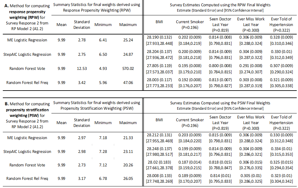
- Table 8. Left Panels: Summary statistics for the final weights derived by applying response propensity weighting (top, A) and propensity stratification weighting (bottom, B) computed from each of the four methods for Survey Response 2 (A1.2). Right Panels: Survey estimates for the five survey outcomes computed using final weights derived by applying response propensity weighting (top, A) and propensity stratification weighting (bottom, B) computed from each of the four methods for Survey Response 2 (A1.2). The standard errors based on bootstrap replication are given in parentheses and 95% confidence intervals are given in brackets below the estimates. The population parameter values for the key outcome variables are also provided under the variable names, for reference.
Putting together estimated biases and standard errors gives the MSEs and design effects displayed in Table 9A for estimates derived using the final sampling weights obtained from each of the four methods using the RPW approach. From this table we see that most of the design effect estimates are near 1 for each outcome and method. However, for each of the five outcomes, estimates generated using the final sampling weights from the random forest rel freq method have consistently smaller design effects compared to those from the other three methods. The MSEs for the estimates produced using the final sampling weights from the random forest rel freq method were smaller or nearly equal to those of any of the methods for four of five survey outcomes. The estimate for current smoker percentage produced from the final sampling weights obtained using the random forest vote method was the smallest of any of the methods. And while the magnitude of the overall MSEs were also small for estimates derived from our sample of respondents identified by Survey Response 2 across the methods and survey outcomes, it is notable to mention that in general the MSEs for the estimates produced using final sampling weights from the random forest rel freq method were between 20 to 80 percent smaller than the MSEs computed from the other three methods across the five survey outcomes. Again, as was the case for Survey Response 1, the magnitude in the reduction for the MSEs using the random forest rel freq method are not inconsequential. substantial and could have practical relevance, especially for studies with smaller budgets or sample sizes.
|
A. Method for computing response propensity weighting (RPW) for Survey Response 2 from RP Model 2 |
Estimated Design Effects and Mean Squared Errors# for Survey Estimates Computed using the RPW Final Weights |
||||
|
BMI |
Current Smoker |
Seen Doctor Last Year |
Ever Miss Work Last Year |
Ever Told of Hypertension |
|
|
ME Logistic Regression |
1.122 |
1.380 |
1.236 |
1.041 |
1.069 |
|
91.38454 |
0.11273 |
0.09134 |
0.11441 |
0.12358 |
|
|
StepAIC Logistic Regression |
1.205 |
1.489 |
1.381 |
1.044 |
1.109 |
|
100.47170 |
0.10221 |
0.10592 |
0.09871 |
0.15772 |
|
|
Random Forest Vote |
0.943 |
1.037 |
1.061 |
0.934 |
0.958 |
|
26.89315 |
0.06279 |
0.43624 |
0.16652 |
0.30701 |
|
|
Random Forest Rel Freq |
0.905 |
1.027 |
0.941 |
0.846 |
0.894 |
|
21.03927 |
0.07819 |
0.09138 |
0.07312 |
0.07331 |
|
|
B. Method for computing response propensity weighting (PSW) for Survey Response 2 from RP Model 2 |
Estimated Design Effects and Mean Squared Errors# for Survey Estimates Computed using the PSW Final Weights |
||||
|
BMI |
Current Smoker |
Seen Doctor Last Year |
Ever Miss Work Last Year |
Ever Told of Hypertension |
|
|
ME Logistic Regression |
1.111 |
1.379 |
1.292 |
1.067 |
1.069 |
|
103.87111 |
0.12324 |
0.09151 |
0.11638 |
0.14873 |
|
|
StepAIC Logistic Regression |
1.208 |
1.466 |
1.407 |
1.059 |
1.125 |
|
127.75968 |
0.09660 |
0.10640 |
0.09412 |
0.24123 |
|
|
Random Forest Vote |
2.200 |
3.632 |
4.072 |
2.773 |
2.866 |
|
43.81405 |
0.28288 |
0.22809 |
0.24681 |
0.24046 |
|
|
Random Forest Rel Freq |
1.158 |
1.554 |
1.715 |
1.219 |
1.165 |
|
25.85973 |
0.13667 |
0.12193 |
0.12278 |
0.09554 |
|
Table 9. Design effects (top number in each cell) and Mean Squared Error estimates (bottom/bold number in each cell) for each of the five survey outcomes using the final sampling weights for each method based on response propensity weighting (top–A) and propensity stratification weighting (bottom–B) for Survey Response 2 (A1.2). # The MSEs presented in this table represent the actual MSE’s multiplied by a factor of 1,000 to illustrate differences.
3.4.2 Final Sampling Weights from the PSW Approach and Resulting Survey Outcome Estimates
The summary statistics for the final sampling weights using the PSW approach for nonresponse adjustment from each of the four methods applied to estimate Survey Response 2 appear to be fairly consistent for the two logistic regression models and the random forest vote method (Table 8B – left panel). Under the PSW approach, the final sampling weights for the random forest rel freq method appear the most variable, and have the largest range of all the methods. However, the smaller range and smaller variability in the final sampling weights from the random forest vote method did not translate into smaller standard errors for the five survey outcome estimates as shown in the right panel of Table 8B. To the contrary, the estimates from the random forest vote method had the highest standard errors among the four methods for every one of the survey outcomes of interest. And while the logistic regression models produced estimates with the smallest standard errors, neither of their 95% confidence intervals for the mean BMI captured the population parameter.
The estimated design effects and MSEs for the estimates derived from final sampling weights from each of the methods are displayed in Table 9B. The design effects for the two logistic regression methods are smaller than those from the estimates from either of the random forest methods. However, unlike for Survey Response 1, the MSEs for estimates obtained from respondents identified by Survey Response 2 for each of the four methods do not exhibit as clear of a pattern across the five survey outcomes. The estimate of BMI produced using the random forest rel freq method has the smallest MSE among all the methods. The estimates produced from either the ME or StepAIC logistic regression methods have the smallest MSE among the four methods for the remaining four survey outcomes. The magnitude of difference in the MSEs across these four survey outcomes for the four methods is smaller than what we observed using the RPW approach for nonresponse weighting for Survey Response 2, however.
4 Discussion and Future Research
We compared logistic regression methods to newer methods based on random forests for creating nonresponse adjustments using both direct propensity adjustments as well as propensity stratification adjustments. Simulated response propensities were generated for each sampled member using both a simple as well as a complex population survey response model (RP Model 1 and 2, respectively). The generated response propensities under the simple and complex scenario were converted into two survey response outcomes that were then modeled using two logistic regression methods as well as two random forest methods. From there nonresponse adjustments based on both direct and propensity stratification approaches were computed using the estimated response propensities from each of the four methods. Final sampling weights from each combination of method and nonresponse adjustment approach were then applied to estimate survey outcomes of interest. We hypothesized that the logistic regression methods would better estimate the propensities generated under the simpler RP Model 1 and thus lead to survey estimates with smaller overall bias and variance. We also hypothesized that the random forest methods would produce better estimates of the propensities generated under the more complex RP Model 2 and that the survey estimates generated using the final sampling weights from these methods would have less bias and variance compared to either of the logistic regression methods.
Our results indicated partial support for both hypotheses. For the first hypothesis we did find that compared to the random forest methods, the logistic regression methods produced estimated propensities that were more highly correlated with those generated under the simple response model. The random forest rel freq method ranked two of the three variables used in the simple population response model among its top three most important predictors whereas the vote method identified only one among its top three important variables. Consequently, the correlation between estimated propensities and those generated by RP Model 1 was higher for the random forest rel freq method compared to the vote method. Better fit to the simple population model for survey response for the logistic regression methods did not imply better overall estimates, however. In fact, the random forest methods produced estimates with the smallest variance and bias for the five survey outcomes under the direct response propensity weighting approach for nonresponse adjustment. Specifically, the rel freq method produced estimates with lowest MSE for three of the five outcomes and the vote method produced estimates with the lowest MSE for the other two outcomes.
For the second hypothesis we found that the correlation between estimated propensities and the propensities generated using the more complex RP Model 2 was highest for the random forest rel freq method and lowest for the random forest vote method. The correlations for the two logistic regression methods fell between these extremes. Under RP Model 2 the random forest methods produced estimates with lower mean squared errors compared to the logistic regression methods for all five survey outcomes. This time, the random forest rel freq method produced estimates with lower MSEs compared to the vote method for four of the five survey outcomes.
When we focus on the propensity stratification approach, the results strongly favor the logistic regression methods under both the simple as well as the complex population survey response model scenarios. The survey estimates derived from the random forest vote method had MSEs that were 1.3 to 4 times larger than those of the estimates obtained from any other method for each of the five survey outcomes under the simple population response scenario. For the complex population response scenario, the MSEs for the estimates obtained from the random forest vote method were between 1.5 and 2.5 times larger than those from the other methods for all outcomes except BMI. The estimates for the proportion of adults told of hypertension produced using the random forest vote method and the StepAIC method had virtually the same MSEs. The relative instability of resulting survey estimates obtained from the random forest vote method using the propensity stratification approach is especially puzzling given that under both the simple and complex population response scenarios, the final sampling weights for the random forest method were the least variable among all the methods. However, the random forest method produced the smallest as well as the largest estimated response propensities under both the simple and complex population response scenarios. In fact, these extreme values were well beyond the corresponding values from the distribution of the response propensities generated from either RP Model 1 or RP Model 2. Another manifestation of instability of the random forest vote method was that the direction of biases in point estimates was reverted when utilizing the response propensity weighting vs. propensity stratification approaches.
The propensity stratification method relies on both respondents as well as nonrespondents in computing the nonresponse adjustments, which in our case was computed as the inverse of the number of respondents to the total number of adults (both respondents and nonrespondents) in each propensity strata. Fluctuations in the bins over the bootstrap replicates can greatly influence the magnitude of the nonresponse adjustments made using the propensity stratification approach. The variability in adjustment factors may in turn result in variability between the resulting survey estimates from one replicate to another and thus impact the overall estimate of sampling error from a replication approach, such as the bootstrap. We note for this study the random forest vote method had the lowest level of consistency in propensity strata assignment for sampled cases across the 500 bootstrap replicates. In particular, under the simple population response scenario, only 34% of the 5,000 cases in our sample were consistently placed in either the same propensity stratum or an adjacent one (up or down) across the 500 bootstrap replications for the random forest vote method compared to 57% for the random forest vote method and 80% for the StepAIC logistic regression method and 99.9% for the ME logistic regression method. Unlike logistic regression, random forests have a random component to them as part of the tree building process and this aspect is a critical part of why they are generally a stronger method for classification problems compared to other tree-based methods. However, this randomness could result in too much noise in the nonresponse adjustment factors and weights across a series of bootstrap replicates that are used to evaluate the sampling errors for survey estimates as we have seen here for the estimates derived from the random forest vote method using the PSW approach for nonresponse weighting. This phenomenon has also been illustrated by Buskirk et al. (2013) who reported higher variability in estimates obtained from random forests compared to logistic regression models across a series of bootstrap subsamples. Adjustments other than the inverse of the response rates within each propensity strata have been used with the propensity stratification approach and these might prove more useful in conjunction with the random forest vote method. One popular approach uses the the inverse of the average of the estimated propensities within each of the propensity strata as the adjustment factor (Valliant and Dever, 2011 and Valliant, Dever and Kreuter, 2013). This approach generally works well in practice if the estimated propensities within each propensity strata are similar (Valliant and Dever, 2011). More research on how the random forest vote method would work with this alternative approach is needed, but given the wider range of estimated propensities obtained from the random forest vote method in this research, we would imagine that such an approach might require more than 5 strata to be effective.
While the random forest vote method does not seem to be well suited for use with the PSW approach for nonresponse adjustment, we have found that the random forest vote and rel freq methods edged out the logistic regression methods using the response propensity weighting approach under both the simple and complex hypothetical population models for survey response. Between the two random forests methods, the rel freq method seemed to edge out the vote method in estimating the generated propensities from both RP Model 1 and 2. Under the RPW approach for nonresponse weighting, the rel freq method also edged out the vote method in terms of the properties of survey estimates under both the simple and complex population survey response scenarios. These results are consistent with the results of Bostrom (2007) who showed that for classification applications, the relative frequency method outperformed the voting method for random forests applied to a wide variety of health and social science data. The primary reason being that the estimated propensities in the rel freq method are based on final nodes that are forced to have a minimum size that is much larger than 1 (the default minimum for the random forest vote method) and thus offer estimates that are more smoothed than the vote method. Possible improvements in the random forest vote method for estimating propensities have been noted by Margineantu and Dietterich (2002) as well as Bostrom (2007) that involve using the entire forest of trees to derive the estimates for each case rather than using only those trees in the forest for which the case is “out of bag”. This process is more consistent with how the two logistic regression methods operationalize estimating response propensities in that the estimated propensity for a given case is based on a model that was estimated using that case. This approach is likely to generate greater differentiation in the response propensity distribution among respondents and nonrespondents, pulling estimated response propensities downward for nonrespondents and upward for respondents. While this separation, as previously mentioned, is likely to generate larger adjustment factors for the lower and upper response propensity strata, stability in the separation of response propensities from respondents and nonrespondents could help improve the quality of resulting survey estimates. More specifically, if this type of separation is stable across multiple iterations of the forest, then it might be completely possible to see reductions in the sampling error for survey estimates derived using sampling weights that contain nonresponse adjustments based on these estimated propensities.
In closing, the random forest rel freq method appears to be a good middle ground alternative to logistic regression for direct propensity adjustments in that it is an automated process, it is nonparametric, in the sense of not making assumptions about the functional form of the response propensity, it can handle complex interactions and associated/correlated predictors and as shown in this research, seems to track well both complex and simple nonresponse mechanisms. As it is with any empirical research though, further work is needed to cross-validate the results we obtained here. While the variables we used to generate the response propensities including age, race, education, income, number of working cell phones, sex have been used in real survey applications for survey weighting adjustments for multiplicity, nonresponse and coverage (Pew Research, 2012 and Pierannunzi, et al., 2012) and others like employment status, prior survey attempts/prior cooperation and phone status have been reported to be related to survey response (Groves, 2006; Steeh and Piekarski, 2008), these are in no way an exhaustive list of candidate predictors. We recognize that our target population, sample and models used to assign response propensities cannot reflect all data sets/target populations, samples and possible response propensity models. While the potential of random forests based on relative class frequencies for nonresponse adjustments using direct propensity weighting seems positive, further work is needed to understand the stability of this method across other finite populations and population response models. Our journey through these forests has just begun!
Appendix 1. Equations for the Response Propensities
Response propensities for RP Model 1 were generated based on the following equation with the coefficients being given on the log odds ratio scale:
![]()
where age is a continuous variable, and race is a categorical variable with 6 categories, including white only, black/African American only, American Indian or Alaskan Native only, Asian only, multiple race, or other. From this equation we see that RP Model 1 generates higher response propensities for those adults who are older, female or white that are consistent with survey response patterns reported in practice (see for example, Pew Research, 2012). For example, the coefficient of +0.48 for sex=females indicates that females are e0.48=1.62 times more likely to respond than not to respond, compared to males, holding all other covariates fixed.
Response propensities for RP Model 2 were generated based on the following equation:
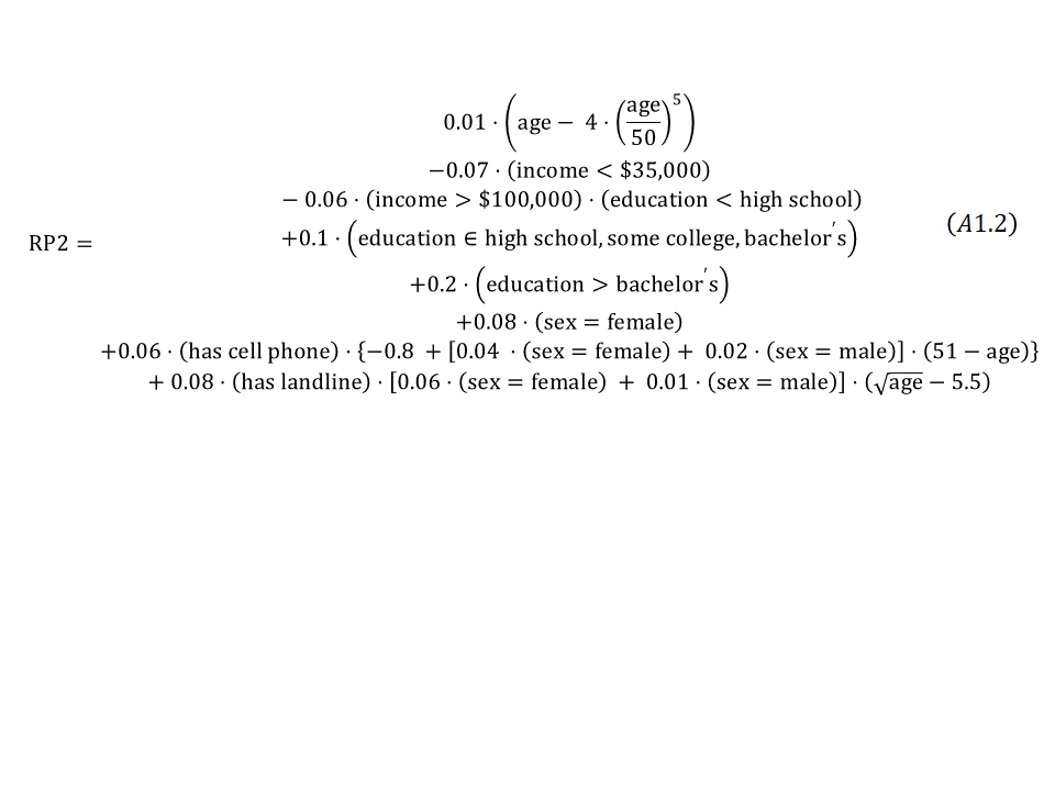
The coefficients in this equation (A1.2) are in absolute terms, so for example, the coefficient of -0.07 for income < $35K indicates that people of this income were on average 7% less likely to respond than people with the same demographics and income $35K to $100K.
Appendix 2. Estimated Models of Survey Response using Our Simple Random Sample
| Predictor Variable | Estimate | Standard Error | P-value |
| (Intercept) | -1.478 | 0.095 | <.00001 |
| sex[Female] | 0.495 | 0.060 | <.00001 |
| wborace[Black] | -0.813 | 0.087 | <.00001 |
| wborace[White] | 0.195 | 0.101 | 0.0544 |
| age_p | 0.030 | 0.002 | <.00001 |
Table A2.1. Coefficients from the model estimating the Survey Response 1 (assigned by RP Model 1) using Stepwise Logistic Regression (AIC-criterion) based on our simple random sample of 5,000 adults.
| Predictor Variable | Estimate | Standard Error | P-Value |
| (Intercept) | -1.578 | 0.156 | <.00001 |
| region[Midwest] | 0.125 | 0.098 | 0.2046 |
| region[South] | 0.124 | 0.089 | 0.1657 |
| region[West] | 0.230 | 0.094 | 0.0145 |
| sex[Female] | 0.656 | 0.171 | <.0001 |
| educ3[Some College] | 0.514 | 0.070 | <.00001 |
| educ3[BS/BA or More] | 1.055 | 0.081 | <.00001 |
| incgrp4[$35,000 – 49,999] | 0.390 | 0.092 | <.0001 |
| incgrp4[$50,000 -99,999] | 0.496 | 0.075 | <.00001 |
| incgrp4[$100,000 and over] | 0.442 | 0.092 | <.00001 |
| age_p | 0.014 | 0.003 | <.00001 |
| sex*age_p | -0.006 | 0.003 | 0.0685 |
Table A2.2. Coefficients from the model estimating Survey Response 2 (assigned by RP Model 2) using Stepwise Logistic Regression (AIC-criterion) based on our simple random sample of 5,000 adults. The coefficients in this table are also based on the log odds scale and as such are not directly comparable to those listed in equation (A1.2). Coefficients in formula A1.2 are based directly on the probability scale.
Appendix 3: Example of a Classification Tree for Predicting Survey Response 1.
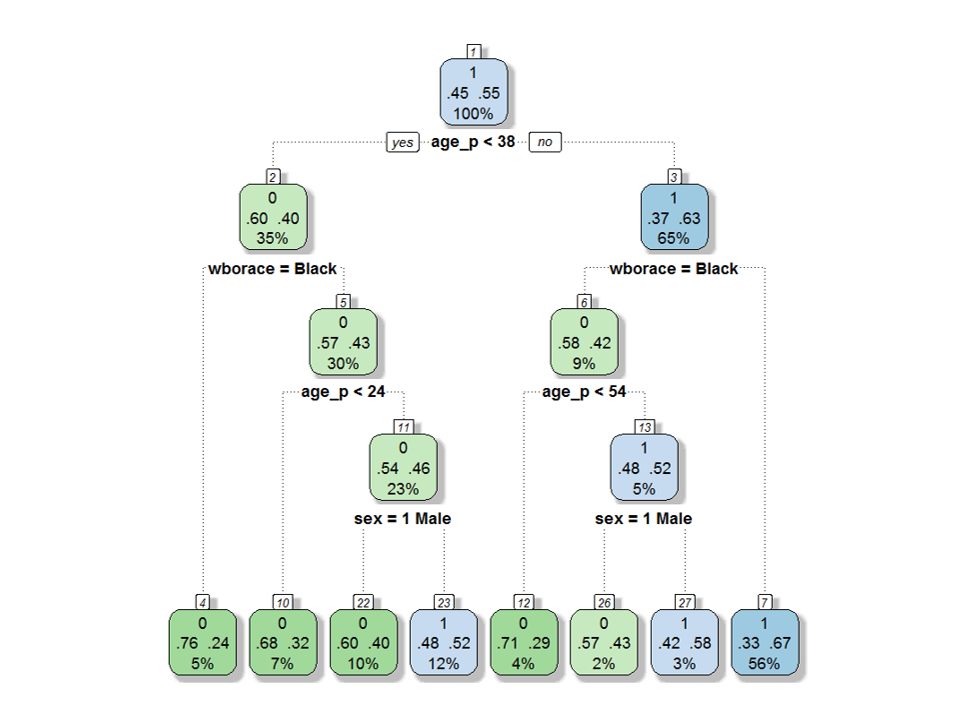
Figure A3. A classification tree for predicting Survey Response 1 from the variables in Table 1.
To determine which node a sampled adult belongs to in the tree, begin at the top and branch downward to the left if the adult satisfies the splitting criterion listed below that node and right otherwise. In the tree in Figure A3 we see that the top split on age_p indicates that the greatest improvement in misclassification errors (which, for an empty tree, or a stump, is simply the smaller of the response rate and 1-response rate) comes from classifying all sampled adults younger than 38 years of age as nonrespondents (green box labeled 2) and those who are 38 years of age or older as respondents (blue box labelled 3). The next split for each of these two nodes is defined by whether or not wborace (race) is “Black.” Black adults who are younger than 38 are classified as nonrespondents and fall into green terminal node number 4. This node is the most homogenous of all 8 terminal nodes given in the tree in Figure 1 with 76% of adults in this node being nonrespondents and the other 24% being respondents. In total, 5% of sampled adults fall into this terminal node. Survey response classification for adults younger than 38 whose race is either “White” or “Other” (i.e. Not “Black”) is further determined by age_p (<24) and then on sex. Using this tree, all sampled adults can be similarly placed into one of the 8 terminal nodes and their predicted category of response or nonresponse from the tree is based on the majority response status of all the adults that share the same terminal node. In this example, terminal nodes that are colored green/blue reflect a prediction of “nonresponse” and “response” for Survey Response 1, respectively.
Appendix 4. Parameter Selection for the Random Forest Models
To determine parameter choices for the random forest models we conducted a preliminary set of tests that generated random forests for each Survey Response outcome using various random seeds. We examined the relationship between variable importance measures for each forest grown using different random seeds as well as error rates as a function of the number of trees in the forest as recommended by Breiman (2001). The tests indicated that stable error rates for the forests should be achieved using 1,000 trees with mtry=3 for both the Random Forest Vote method as well as the Random Forest Rel Freq method for each of the Survey Response outcomes. Additionally, our preliminary tests for the node size parameter used for the relative frequency method indicated increasing the value from 5 to 20 for estimating both Survey Response 1 and 2. The mtry parameter value represents one less than the default used for regression (i.e. Random Forest Rel Freq method) and is equal to the default used for random forests for classification (i.e. binary outcomes). Our preliminary tests for the random forest rel freq method revealed lower error rates using a smaller value of mtry (3 compared to 4). The number of trees used in both random forest methods represents double the default value of 500.
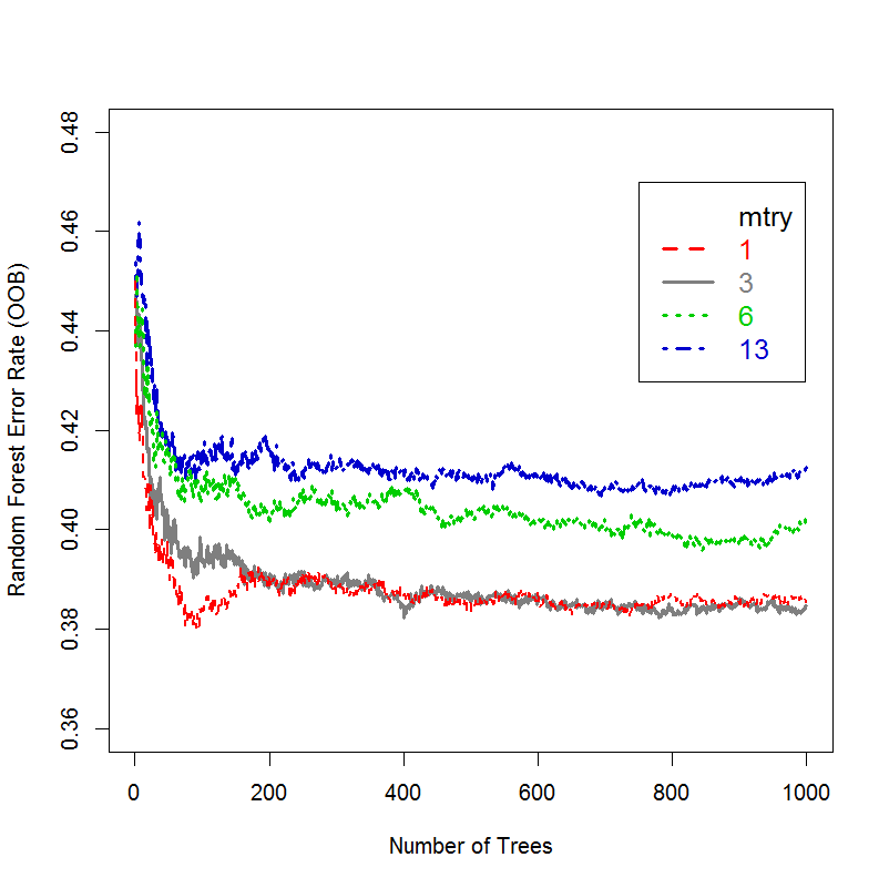
Figure A4: Random forest error rates (derived from out of bag cases) as a function of the number of trees for various values of the mtry parameter based on the random forest vote method applied to estimate Survey Response 1 in preliminary testing.
In Figure A4, the estimated prediction error rate for the random forest vote method applied to Survey Response 1 is plotted as a function of the number of trees in the forest for the default value of mtry as well as other commonly used values including 1, 6 and 13 corresponding to p/2 and p, respectively (Breiman, 2001). From this figure it can be seen that the error rates, regardless of the mtry parameter, generally decrease as the number of trees increases and stabilize after about 800 trees. The prediction error rates for mtry=1 and mtry=3 are very similar and are slightly less than the error rates for random forests run using mtry=6 and mtry=13. While it is clear from Figure A4 that the error rates improve little for forests that use more than 800 trees, we used 1,000 trees in each of the final forest models to improve the stability of the propensity estimates derived from the voting method because these propensities are estimated using only the trees in the forest for which the given sampled adult is out of bag. So in our case a forest with 1,000 trees implies that propensity estimates are derived using roughly 320 trees per sampled adult, on average. The prediction error rate results for the random forest vote method applied to estimating Survey Response 2 were similar and are not shown.
Appendix 5. Standard Error Calculation Methodology
To compute standard errors for the estimates, we used a separate set of 500 bootstrap replicates (Rao and Wu, 1988) for each of the Survey Response outcomes. To form a survey bootstrap replicate, a sample of 4,999 was selected with replacement from the entire original sample of 5,000 adults. Using each of the 500 bootstrap samples in the first set, each of the four methods were applied to estimate Survey Response 1. Nonresponse adjustments were then applied based on the estimated response propensities each of the methods using both the RPW and PSW approaches. Within each bootstrap replicate eight final sampling weights were created – two per estimation method corresponding to direct and propensity adjustments. A Final scaling factor so that the sum of the final weights equaled the finite population size) was also applied to each final bootstrap replicate to ensure the final weights summed to the finite population size. This process was repeated for Survey Response 2 using the second set of independently generated bootstrap replicates.
While the Taylor series linearization method is most commonly used for variance estimation in surveys (Wolter 2007), it relies on certain smoothness assumptions that discrete choice models such as classification trees (and by extension, random forests) do not satisfy. Hence replicate weight methods, such as the bootstrap, need to be used that allow us to understand the impact of all the weighting adjustment steps on the final variance of the survey estimates (Chowdhury, 2013, Shao, 1996 and Kolenikov, 2010).
Appendix 6. Acronyms and notation
| AIC | Akaike information criterion (Sec. 2.3.1) |
| AUC | Area under receiver operating characteristic curve (Sec. 3.1) |
| BMI | Body mass index (Sec. 2.4) |
| ME-logistic | Main effect logistic regression model (Sec. 2.3.1) |
| NHIS | National Health Interview Survey (Sec. 2.1) |
| PSW | Propensity stratification weighting (Sec. 2.4) |
| CART | Classification and Regression Trees (Sec 2.3.2) |
| Random Forest vote | Random forest vote method (Sec 2.3.2) |
| Random Forest rel freq | Random forest relative frequency method (Sec. 2.3.2) |
| RP Model 1, 2 | Response propensity models (Sec. 2.2) |
| RPW | Response propensity weighting (Sec. 2.4) |
| StepAIC | AIC-based stepwise selection of the main effects followed by selection of interactions in logistic regression model (Sec. 2.3.1) |
References
- Agresti, A. and Coull, B.A. (1998). Approximate is Better than “Exact” for Interval Estimation of Binomial Proportions. The American Statistician, 52(2), 119-126.
- Akaike, H. (1974). A new look at the statistical model identification. Automatic Control, IEEE Transactions on 19 (6), 716-723.
- Allison, P. (2008) Convergence Failures in Logistic Regression. Proceedings of the SAS Global Forum, Paper 360. Available at: http://www2.sas.com/proceedings/forum2008/360-2008.pdf, accessed January 15, 2015.
- Ayer, T., Chhatwal, J., Alagoz, O., Kahn, C. E., Woods, R. W., & Burnside, E. S. (2010). Comparison of Logistic Regression and Artificial Neural Network Models in Breast Cancer Risk Estimation. Radiographics, 30(1), 13–22. doi:10.1148/rg.301095057.
- Bethlehem, J.G., (2002). Weighting Nonresponse Adjustments Based on Auxiliary Information (Survey Nonresponse, Chapter 18, Edited by Groves et al.) Wiley, Ney York.
- Bethlehem, J., Cobben, F. and Schouten, B. (2011). Handbook of Nonresponse in Household Surveys. Wiley, Hoboken.
- Bostrom, H. (2007) Estimating Class Probabilities in Random Forests. Machine Learning and Applications – Proceedings of the Sixth International Conference on Machine Learning and Applications, Cincinnati, Ohio, 211 – 216. Available at http://people.dsv.su.se/~henke/papers/bostrom07c.pdf
- Breiman, L. (2001). Random Forests. Machine Learning, 45 (1), 5-32.
- Breiman, L., Friedman, J., Stone, C.J. and Olshen, R. A. (1984). Classification and Regression Trees (1 ed.). Chapman & Hall/CRC, Boca Raton.
- Brick, J.M. (2013). Unit Nonresponse and Weighting Adjustments: A Critical Review. Journal of Official Statistics, Vol. 29(3), 329-353.
- Burks, A.T. and Buskirk, T. D. (2012). Can Response Propensities Grow on Trees? Exploring Response Propensity Models Based on Random Forests Using Ancillary Data Appended to an ABS Sampling Frame. Paper presented at the 2012 Midwest Association of Public Opinion Research, Chicago, IL. http://www.mapor.org/confdocs/progarchives/mapor_2012.pdf (accessed on March 10, 2014).
- Buskirk, T. D., Burks, A-T., West, B.T. (2013) “Can Survey Response Propensities Grow on Trees? Comparing the Validity of Random Forests and Logistic Regression Models Using Population Variables Appended to an ABS Sampling Frame,” Poster presented at the 2013 Conference on Statistical Practice, New Orleans.
- Chen, Q., Gelman, A., Tracy, M., Norris, F. H., & Galea, S. (2012). Weighting Adjustments for Panel Nonresponse. Available at http://www.stat.columbia.edu/~gelman/research/unpublished/weighting%20adjustments%20for%20panel%20surveys.pdf , accessed on July 22, 2014.
- Chowdhury, S. (2013) A Comparison of Taylor Linearization and Balanced Repeated Replication Methods for Variance. Agency for Healthcare Research and Quality Working Paper No. 13004 Available at: http://meps.ahrq.gov/mepsweb/data_files/publications/workingpapers/wp_13004.pdf (accessed July 22, 2014).
- David, M., Little, R. J. A., Samuhel, M. E., and Triest, R. K. (1983). Nonrandom nonresponse models based on the propensity to respond, Proceedings of the Business and Economic Statistics Section, American Statistical Association, 168-173.
- Da Silva, D.N. and Opsomer, J.D. (2009). Nonparametric Propensity Weighting for Survey Nonresponse through Local Polynomial Regression. Survey Methodology, 35, 165-176.
- Goldstein,B.A., Polley, E.C. and Briggs, F.B.S. (2011). Random forests for genetic association studies. Statistical Applications in Genetics and Molecular Biology, 10(1):32.
- Groves, R. M. (2006). Nonresponse rates and nonresponse bias in household surveys. Public Opinion Quarterly 70 (5), 646-675.
- Harrell, F. (2010), Regression Modeling Strategies: With Applications to Linear Models, Logistic Regression, and Survival Analysis, 2nd Ed, Springer-Verlag, New York.
- Hastie, T., R. Tibshirani, and J. Friedman (2009). The Elements of Statistical Learning. 2nd edition. New York: Springer-Verlag.
- James, G., Witten, D., Hastie, T. and Tibshirani, R. (2013). An Introduction to Statistical Learning with Applications in R. New York: Springer.
- Kalton, G., & Flores-Cervantes, I. (2003). Weighting Methods. Journal of official statistics, 19(2), 81-97.
- Kish, L. (1965). Survey Sampling. John Wiley & Sons, Inc., New York, London.
- Kolenikov, S. (2010). Resampling variance estimation for complex survey data. The Stata Journal 10 (2), 165-199.
- Kreuter, F. (Editor) (2013). Improving Surveys with Paradata: Analytic Uses of Process Information. Wiley, New York.
- Little, R.J.A. (1986). “Survey Nonresponse Adjustments for Estimates of Means.” International Statistical Review, vol. 54, 1986, pp. 139-157.
- Little, R. J. & Vartivarian, S. (2003). On weighting the rates in nonresponse weights. Statistics in Medicine, 22(9), 1589–1599.
- Little, R.J.A, and Vartivarian, S. (2005). Does Weighting for Nonresponse Increase the Variance of Survey Means? Survey Methodology, 31(2), 161-168.
- Margineantu, D. D. and Dietterich, T. G. (2002) Improved class probability estimates from decision tree models. in D. D. Denison, M. H. Hansen, C. C. Holmes, B. Mallick, and B. Yu (Eds.) Nonlinear Estimation and Classification; Lecture Notes in Statistics, 171, pp. 169-184. New York: Springer-Verlag.
- McCarthy, J.T., Jacob, T. and Atkinson, D. (2009). Innovative Uses of Data Mining Techniques in the Production of Official Statistics. Federal Committee on Statistical Methodology Papers, accessed from http://www.fcsm.gov/09papers/McCarthy_X-A.pdf, April 1, 2014.
- Meekins, B. J., & Sangster, R. L. (2004). Predicting wave nonresponse from prior wave data quality. In Proceedings of the Annual Meeting of the American Statistical Association.
- Mendez, G., Buskirk, T.D., Lohr, S. and Haag, S. (2008). Factors Associated with Persistence in Science and Engineering Majors: An Exploratory Study Using Random Forests. Journal of Engineering Education, 97(1), 57-70.
- Pal, M., 2005. Random forest classifier for remote sensing classification. International Journal of Remote Sensing, 26(1), 217–222.
- Phipps, P. and Toth, D. (2012). Analyzing Establishment Nonresponse Using an Interpretable Regression Tree Model with Linked Administrative Data. Annals of Applied Statistics, 6, 772-794.
- Pierannunzi, C., Town,M., Garvin, W., Shaw, F.E. and Ballus, L. (2012). Methodologic Changes in the Behavioral Risk Factor Surveillance System in 2011 and Potential Effects on Prevalence Estimates, Morbidity and Mortality Weekly Report, 61(22), 410-413.
- Rosenbaum, P. R., and Rubin, D. B., (1983), The central role of the propensity score in observational studies for causal effects,” Biometrika, 70, 4155.
- Rao, J. N. K. and C. F. J. Wu (1988). Resampling inference with complex survey data. Journal of the American Statistical Association, 83 (401), 231-241.
- Segal, Mark R. (2004). Machine Learning Benchmarks and Random Forest Regression. Center for Bioinformatics & Molecular Biostatistics. UC San Francisco: Center for Bioinformatics and Molecular Biostatistics. Retrieved from: https://escholarship.org/uc/item/35x3v9t4 , January 20, 2015.
- Shao, J. (1996). Resampling methods in sample surveys. Statistics 27, 203-254.
- Steeh, C. and Piekarski, L. 2008. “Accommodating New Technologies: Mobile and VoIP Communication.” In Advances in Telephone Survey Methodology edited by James M. Lepkowski, Clyde Tucker, J. Michael Brick, Edith de Leeuw, Lilli Japec, Paul J. Lavrakas, Michael W. Link, and Roberta L. Sangster. New York: Wiley; 423-448.
- Strobl, C., Boulesteix, A-L., Zeileis, A. and Hothorn, T. (2007). Bias in Random Forest Variable Importance Measures: Illustrations, Sources and a Solution. BMC Bioinformatics, Vol. 8 (25).
- Valliant, R. and Dever, J. (2011). Estimating Propensity Adjustments for Volunteer Web Surveys. Sociological Methods & Research, 40(1), 105-137.
- Valliant, R., Dever, J., and Kreuter, F. (2013). Practical Tools for Designing and Weighting Survey Samples. Springer, New York.
- Wolter, K. M. (2007). Introduction to Variance Estimation (2nd ed.). New York: Springer.
- Yamamura, K. (1999). Transformation using (x + 0.5) to stabilize the variance of populations. Researches on Population Ecology, 41(3), 229-234.
-
Keywords
calibration CATI coverage coverage bias cross-national surveys data linkage data quality European Social Survey experiment face-to-face face-to-face survey Facebook hard to reach populations incentives item nonresponse measurement measurement error mixed-mode surveys multitasking non-probability samples Nonresponse nonresponse bias nonresponse rates paradata PIAAC Probability sample probability samples QR codes rare populations response rate Satisficing social desirability Social media survey survey-taking climate survey data survey management survey methods Telephone survey telephone surveys total survey error unit nonresponse validity web survey Web surveys weighting