Possible Uses of Nonprobability Sampling for the Social Sciences

---

Abstract

This paper compares the usability of data stemming from probability sampling with data stemming from nonprobability sampling. It develops six research scenarios that differ in their research goals and assumptions about the data generating process. It is shown that inferences from data stemming from nonprobability sampling implies demanding assumptions on the homogeneity of the units being studied. Researchers who are not willing to pose these assumptions are generally better off using data from probability sampling, regardless of the amount of nonresponse. However, even in cases when data from probability sampling is clearly advertised, data stemming from nonprobability sampling may contribute to the cumulative scientific endeavour of pinpointing a plausible interval for the parameter of interest.

Keywords

Causal Inference, Descriptive Inference, Fit-for-purpose, Interactions, Nonprobability sample, PATE, Probability sample

Acknowledgement

The paper is a shortened version of related talks at the InGRID2 WageIndicator Data Forum on 31 August 2017 in Amsterdam, and at the symposium of the of the platform for surveys, methods and empirical analysis (PUMA) in Linz, Austria on 13 October 2017. I wish to thank the participants of these conference for their comments and critical remarks.

1 Introduction

The aim of this paper is to contribute to the debate about non-statistical notions of survey quality (e.g., fit for purpose, etc.; see Groves et al., 2009, pp. 62—63). More specifically, the paper seeks to give tentative answers to the following question: What kind of purposes allow for deviation from the gold standard of surveys on target persons selected by probability samples? To this end it develops a typology of “research scenarios” defined by the goal of the research and assumptions about the nature of the units being studied. It is proposed that these research scenarios differ in the amount of robustness against deficiencies that may arise from nonprobability sampling.

It is important to understand that this paper deals with the sampling method, as opposed to the sample characteristic. The paper uses the term probability sample (PS) for samples with known or estimable sampling probabilities. A nonprobability sample (NPS), then, is a sample with sampling probabilities that cannot be estimated with a reasonable degree of precision. From these characteristics of the sample, the method of sampling should be kept separate. Probability sampling (PSg) is a method that leads to a PS, if successful. However, in practice, PSg is rarely successful due to coverage errors, selection errors and nonresponse errors (Groves & Lyberg, 2010, p. 856); thus data from PSg may end up having similar inference quality to that from NPSg. Likewise, NPSg is a sampling design¹ that usually leads to a NPS, although clever weighting may enable the actual data to achieve the inference quality of a PS.

Empirical evidence suggests that data stemming from deficient PSg provides more accurate results than data from NPSg, even if the latter is analysed with profound statistical sufficiency (Scherpenzeel & Bethlehem, 2011; Yeager et al., 2011; MacInnis, Krosnick, Ho, & Cho, 2018; Sohlberg, Gilljam, & Martinsson, 2017; Sturgis et al., 2018). However, this is not the topic of this paper. Instead the paper asks whether NPSs may still be usable for certain research questions. Or, more specifically, what assumptions about the data generating process must be applied to justify the use of data from NPSs.

Throughout the paper, the formal notation is kept as minimal as possible. The aim is to provide an intuitive understanding of the topics discussed. A more thorough treatise on a related topic is given by Kohler, Kreuter, and Stuart (2019), from which I borrowed the differentiation between the sample characteristic and the sampling method, as well as the recommendations in Section 4. The major contribution of the present paper is to systematically link these recommendations to the typology of research scenarios.

The paper proceeds as follows. Section 2 develops six major research scenarios. For each of the research scenarios the consequences of NPSg are then discussed (Sec. 3). The discussion will show that PSg has advantages for only two of the six scenarios, and Section 4 will provide some ideas about how data from NPSg may be used for the remaining scenarios.

2 Research scenarios

This section develops six research scenarios that differ in the usability of NPS data. The typology is developed here, while the consequence of nonprobability sampling for each type is discussed in Section 3. A graphical display of the typology is given in Figure 1.

2.1 Descriptive vs. Causal Inference

It is common to distinguish descriptive and causal inferential research questions (King, Keohane, & Verba, 1994, pp. 34—109). Descriptive inferential research strives to give a statistical summary of all units that exist in a well-defined finite population using the data at hand. Three examples of descriptive research questions are:

1. “What is the proportion of partisans for party A in the electorate of country B in year C?”
2. “How big is the difference in partisanship for party A in the electorate of country B in year C between blue and white collar employees?”
3. “How did the difference between blue and white collar employees regarding their partisanship for party A in the electorate of B change over the last t years?”

The statistic of interest for the first research question is the proportion of partisans for party A, and the finite population is the electorate of country B in year C. Readers should be aware that this research question includes the standard research question of the polling industry, i.e. the prediction of an election result. Of course, it also includes any research questions that involve predictions of some outcome for a defined population. The second example asks for some measure of association between class and voting behaviour, e.g. the Alford Index of class voting (Alford, 1962), a regression coefficient of a multinomial logistic regression of voting behaviour on social class, etc. Finally, the third example might be studied with the interaction term between time and social class in a regression for partisanship. Here, the finite population is the electorate of all the years under study.

In all these examples the research interest is essentially on the finite population. We are not interested here in the value of a single person, but in a summary of many of them. The values of the single persons are an input to this description but do not have a value of their own.

Causal inferential research questions strive to estimate the causal effect as defined by the counterfactual concept of causality, which is also known as the potential outcome framework, or Rubin Causal Model (Neyman, Iwaszkiewicz, & Kolodziejczyk, 1935; Rubin, 1974). According to this concept, the causal effect (hereafter: treatment effect, ) of some treatment on some outcome for the unit is defined as the difference between the value of under the condition that the unit receives the treatment and the value of under the condition that did not receive the treatment, formally:

(1)  

At this point the research question still remains on the treatment effect for one single unit, as in the following examples:

1. “Did Peter’s blood pressure decrease because he took Bidil?”²
2. “Did Paul win the election because he was the incumbent?”³
3. “Did Mary fail her math exam because she had math lessons together with boys?”⁴

Of course, none of these questions can be answered. It is well known that the treatment effect for the single unit is inherently not observable because one cannot observe the counterfactual outcome. What would have happened if Peter had not taken Bidil? What would the election result have been if Paul had been a new candidate? Would Mary have passed the exam if she had been in a school for girls? None of these potential outcomes can be observed if reality treated Peter, Paul, and Mary differently. In practice therefore other observations⁵ are needed to make a statement about the treatment effect for unit .

Note carefully, the different role of single units for causal and descriptive inference. While descriptive inference requires single units as input for the description of the population, causal inference uses single observations to infer about the process that generated the outcome for one specific unit. For causal research, there isn’t a population to infer to, but a data generating process. And this inference to a data generating process can be of interest even if it is about the data generating process for one single unit—as the examples illustrate.

In practice, of course, social scientists usually study the treatment effect for more than one unit. In this case, however, it becomes important whether or not the treatment effects of the units differ between each other. This is discussed in greater detail in the next subsection.

2.2 Homogeneity vs. Heterogeneity

The second dimension of the typology of research scenarios arise from assumptions about the homogeneity of the population. For descriptive inference, a population can be considered homogeneous if the parameter of interest is identical for each possible grouping that is not a function of the parameter of interest itself. For the first example of the previous subsection, this assumption would hold if the proportion of partisans for party A were identical for men and women, rich and poor, old and young, or any other grouping that is not a function of partisanship itself. Equivalently, for the second example the population is homogeneous if the Alford Index were the same for men and women, rich and poor, and so forth. An extreme form of homogeneity is a population with all units being identical.

For causal inference, homogeneity means that the treatment effect is the same for all units, regardless where and when the treatment takes place. In terms of example 4 of the previous subsection: The treatment effect of Bidil would be homogeneous if human beings—at all times and in all places—would respond with a decrease of blood pressure in consequence of taking Bidil. Likewise co-education might decrease the probability of failing an exam by the same amount for all girls—everywhere and every time.

Whether homogeneity can be assumed depends on the research question at hand, and on the definition of the units a researcher is inferring to. This is true for both descriptive and causal research. It is known, for example, that partisanship differs strongly between social strata in most countries, which renders a homogeneity assumption for example 1 ludicrous. For the description of associations (example 2), the situation changes a bit. Of course, it would be too bold to assume that the partisanship of blue and white collar workers differ by the same amount for all possible groupings, but at least it seems fair to assume that left-wing partisanship is stronger among blue collar employees than among white collar employees. The assumption might become even more plausible if a researcher restricts the inference population to, say, older men in big German cities. For causal research, the plausibility of the homogeneity assumption also depends on the research question and the units the researcher is inferring to. The causal effect of co-education on girls’ math performance very plausibly differs between pupils due to their individual or school characteristics. The effect of Bidil on blood pressure, on the other hand, might be homogeneous at least in the sense that blood pressure is always decreased. In the latter case the homogeneity assumption might become even more plausible if the inference is restricted to a specific genotype, African Americans, for example.

The last example points to a differentiation that needs to be addressed only for causal research, and only in presence of heterogeneity. If treatment effects could be assumed to be homogeneous, it would be enough to estimate the treatment effect for one single arbitrarily selected unit. The results would then be generalisable directly to other units. If, on the other hand, individual treatment effects differ between units, direct generalisation will not be possible.⁶ Before going on, causal researchers in such cases thus must refine their research question.

2.3 Causal research question refinement

One possible refinement of the research question is to isolate a special population for which the homogeneity assumption holds. This might seem a bit superficial, but there are instances where such a strategy is sensible. For medical doctors it might be helpful to know that a medical drug decreases the blood pressure of persons of a specific genotype. If doctors knew that, they could cure—at least—these persons. Similarly, if we knew that co-education hampers girls’ math performance in public elementary schools, this knowledge could be helpful for creating an environment without disadvantages for girls.

A second refinement is to study an interaction. Studying interactions means to find out why the treatment effects differ between units. Essentially, the task now is to differentiate the units into special populations that differ in their treatment effects. The characteristic that is being used for the definition of the special populations may then be taken as a a candidate for the cause of the heterogeneity.

The third possible refinement is to present some kind of a summary statistic of the heterogeneous treatment effects. In practice, the most frequently used summary statistic for this purpose is the arithmetic mean, which leads to the so called “population averaged treatment effect” (PATE; see Imai, King, & Stuart, 2008). However, other summary statistics are conceivable as well (e.g. quantiles, variance, etc.). In any case, the interest in a summary statistic of the treatment effects pushes causal researchers towards the logic of a description: They describe the distribution of the individual treatment effects for a finite population.

The statistical literature on causal research often focuses on the PATEs (Winship & Morgan, 1999, p. 664). This may lead scientists to concentrate on studying the PATE and to leave the other refinements aside. However, as Kohler et al. (2019) states, this should not be an automatic reaction to heterogeneous treatment effects. Consider a case in which a treatment has positive effects on some people and negative effects on others. A policy recommendation should, then, not recommend one policy for all individuals just because it helps on average. Instead, statements about which persons, or under what conditions, a policy helps are required. “Scenarios in which the PATE would be of interest include settings where health insurance companies might be interested in whether a new medical drug cures a disease better on average than the established alternative, or a state policymaker wanting to predict average effects if a new policy is implemented for all individuals within the state. Also, if a researcher did not have data on variables that interact with the treatment variable of interest, the estimation of the PATE would be a sensible fallback solution” (Kohler et al., 2019, p. 10.16).

The next section discusses the consequences of NPS data for each of the six research scenarios. Before doing so, some remarks about the frequency of the various research questions are offered. While I am not aware of an empirical study about the distribution of research scenarios, it must be stressed that both, official statistics and the polling industry, are engaged in descriptive research of Type 2a, so this research scenario is definitely highly relevant. The same is also true for causal research questions in general. A review of two volumes of the European Sociological Review shows that a large majority of sociological research deals with causal research questions (Kohler, Sawert, & Class, 2019), and “causal inference has always been the name of the game in applied econometrics” (Angrist & Pischke, 2009, p. 113). However, I have the impression that the role of homogeneity assumptions are often neglected in causal research applications, particularly in the field of experimental economics. For individual researchers it is however of little importance what kind of research the majority of studies apply. The only important question is what kind of research scenario they are operating in.

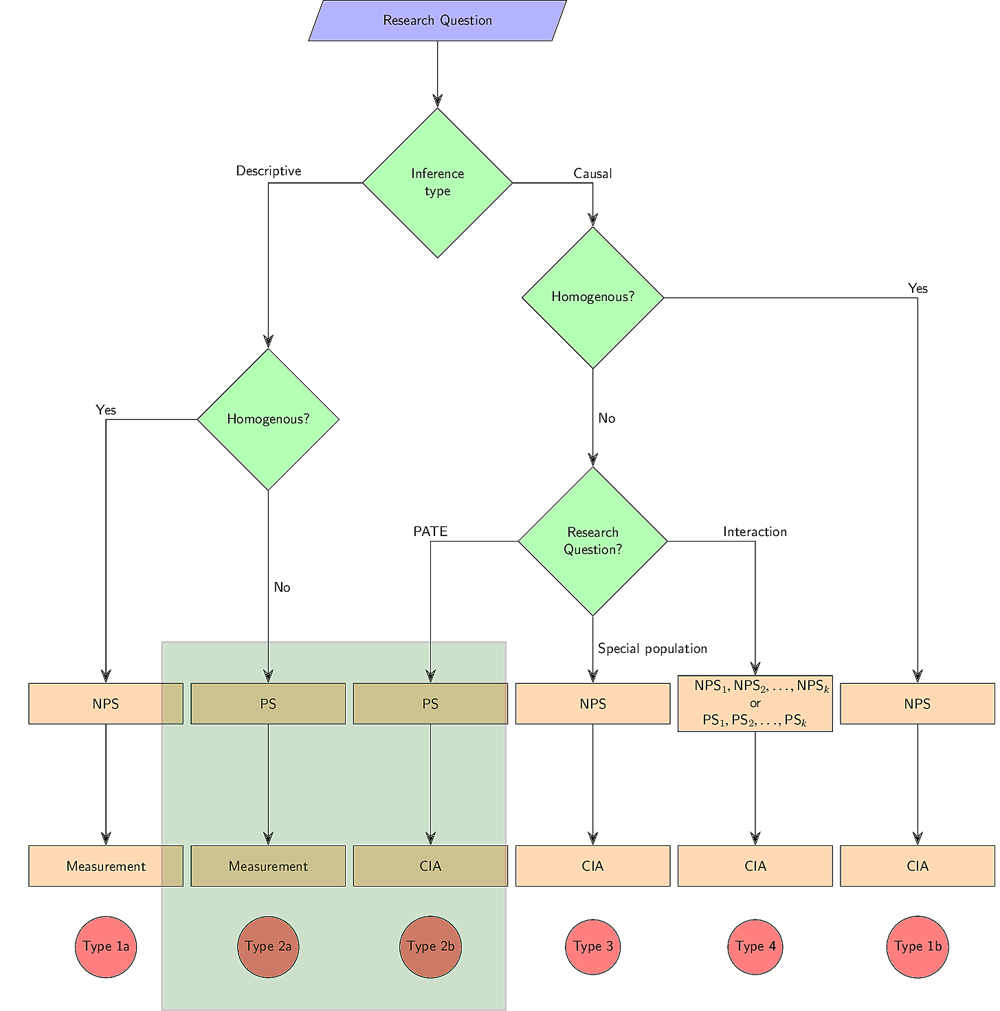
3 Consequences of NPSg

Using characteristics of the research questions and assumptions of the nature of the unit one is inferring to, the previous section distinguished six typical research scenarios. In Figure 1 these types are marked with names “Type 1” to “Type 4”, with Types 1 and 2 being subdivided into variants a and b. In this section, I discuss—for each major scenario—the consequence of NPSs in terms of the bias⁷. To this end, I rely on the formula for the self-selection bias of the calculated sample mean as presented by Bethlehem, Cobben, and Schouten (2011, p. 44). The formula assumes a sampling method with possibly varying selection probabilities and no other errors than selection errors. Using Taylor linearization, the bias of the mean then is

(2)  

with denoting the individual selection probabilities. is the correlation between the probability that a unit is selected (or selects him/herself) and the variable of interest. If respondents participate in a survey because they want to influence the survey results, this term becomes large; see Bethlehem (2015) for a real world example in which a pastor recommended a congregation to participate in an online survey to prevent new legislation on Sunday shopping. More generally, is nonzero whenever a factor that affects the selection also affect the values of the variable of interest. is the standard deviation of the variable in the population, and thus basically a measure for the amount of heterogeneity. is the standard deviation of the individual selection probabilities. It is zero if all units are selected with the same probability. For NPSg it seems only theoretically possible that . The denominator of equation (2) refers to the mean of the individual selection probabilities, which can be estimated with

(3)  

Here, is the number of observed units and is the size of the population. Thus, the bias of the mean from data stemming from NPSg depends on the population size and the sample size. The larger the population, and the smaller the number of observed units, the larger the bias.

Of course, the self-selection bias is not the only source of bias in empirical research. For descriptive research, measurement errors (Groves & Lyberg, 2010, p. 856) are an important source of bias, and for causal research the conditional independence assumption (CIA) must hold. For simplicity the following discussion assumes that these problems are solved.

3.1 Types 1a and 1b

The homogeneity assumptions applied for Types 1a and 1b translate to for 1b, and for Type 1a. As a consequence, the self-selection bias is always zero under those scenarios. If units are homogeneous, the sampling design does not matter at all.

Of course the statement that sampling design does not matter critically hinges on the validity of the homogeneity assumption. It has been mentioned already that the plausibility of this assumption depends on the research question at hand. For most, if not all, descriptive research questions, the homogeneity assumption is only a limiting case without practical relevance. For causal research it is more often accepted, at least implicitly. By and large, the homogeneity assumption is applied whenever experimental researchers trust the external validity of their internally valid results gained from special populations. In fact, the experiments on highly selective student samples that form the backbone of many experimental research designs often rely on the assumption that the treatment effect is a function of the treatment and not a function of the students they treat.

3.2 Types 2a and 2b

For research scenarios 2a and 2b, the term in the numerator of equation (2) is assumed to be larger than zero. Thereby, the only difference between scenarios 2a and 2b is that the term refers to the mean of some arbitrary individual characteristic in the former, and to the mean of the individual treatment effects in the latter. The consequences of NPSg are the same for both designs: As , the results are biased
if neither , nor are zero, which usually
applies to NPSg.

The size of cannot be controlled completely by the research design. Of course, would be zero if all units of the finite population were selected with the same probability, i.e., for simple random samples (SRSs). However true SRSs are practically impossible. For PS it would be possible to correct estimators such that , but we assume here that true PSs also do not exist in practice. If the units are selected by NPSg, the size of the nominator in equation (2) becomes solely a function of the characteristic of the inference population. A researcher that wants to minimise the bias thus should consider measures to increase the size of the denominator.

Treating the nominator of equation (2) as a fixed characteristic of the inference population, the amount of bias depends on the mean of the individual selection probabilities. In a nonprobability sample, the mean selection probability boils down to the number of observations divided by the population size; see equation (3). In the standard case of a large population, this is a very small number—even in cases of so called “big data”. Of course, if the population is small, it will become feasible to observe a large proportion of it, so that the size of the bias might become acceptable⁸.

However, a more general way to minimise the bias for studies that fall into the categories of Type 2a or 2b is to use PSg. As mentioned above, it is possible to correct the formulas for many descriptive statistics to reflect unequal sampling probabilities. For the most basic case of a simple random sample, with equal selection probabilities for all units, and nonresponse as the only source of bias, the simple random sampling equivalent of the self-selection bias is

(4)  

with being each unit’s response probabilities given that it
is sampled, and being their mean (for details see Bethlehem, 1988). The latter can be estimated using the sample’s
response rate, i.e.

(5)  

with being the number of units that are sampled but not observed. Here, the population size is no longer part of the definition of bias, and also the sample size does not play a role. Thus, the nonresponse bias under PSg will be smaller than the self-selection bias under NPSg for most practical situations. In addition, the advantage of PSg will be likely to be even larger because is limited to some degree by the sampling design; i.e., in many cases. Of course, the bias can be further reduced when a weighting adjustment is used to compensate for the missing data by modelling the unknown nonresponse mechanism. In all those regards PSg has many advantages over NPSg, despite nonresponse. Put differently, for research scenarios 2a and 2b, it is usually better to have deficient data from a PS, than to have data from a large NPS. Section 4 will show how data from NPSg might nevertheless contribute to research under scenario 2.

3.3 Type 3

Research scenario 3 assumes that term . Provided that the units stem from the sub-population in question, sampling does not matter. In this regard the situation is identical to research scenario 1b above.

However, there is a thin line between research scenarios 3 and 1b: For Type 1b, the researchers must assume that the treatment effect as such is homogeneous, while for Type 3 the researchers assume the opposite, and thus seek to specify a sub-population for which homogeneity can be assumed. A consequence of this is that researchers under scenario 3 cannot generalise the findings to arbitrary populations. The inference of the Type 3 researcher is restricted to the special population for which homogeneity can be assumed.

3.4 Type 4

Research scenario 4 asks for reasons for heterogeneous treatment effects. Obviously this research question already implies heterogeneity of treatment effects. Researchers that are able to stratify the population based on all reasons for the heterogeneity end up with several special populations that are homogeneous within and heterogeneous between. As for each special population, researchers could then arbitrarily select units for each special population. The statistic of interest would then be the difference of the treatment effects between the various special populations.

Research scenario 4 is also perceivable under heterogeneity for each special population. In this case, the researchers are forced to summarise the treatment effects for each special population. As for any of them, researchers are pushed into scenario 2b for each special population. That is to say, the researcher should select, for each special population, the units such that the distribution of the individual treatment effects of the sampled units reflects the population’s distribution of the individual treatment effects in a known way. As discussed in subsection 3.2, PSg is a powerful measure to this end.

4 Uses of nonprobability samples

The previous section has shown that NPSg can be readily used for research scenarios 1a, 1b, 3 and, perhaps, 4. The common ground of these scenarios is that they rely on a homogeneity assumption. Researchers who are using nonprobability samples should be aware of this, and should make this assumption stand out. It goes without saying that this will invite criticism, but this is considered an advantage here.

However, one of the most useful possible applications of data from NPSg is to actually examine the homogeneity assumption. Consider experimental economists who study some (causal) parameters in a computer lab with their faculty’s students. Assuming homogeneity, they could infer their estimated treatment effects to all human beings (scenario 1b). But is the homogeneity assumption correct? It will be hard to determine this based on the experiments alone. But if researchers were willing to re-run the experiment with arbitrarily selected persons that are very different to their students, evidence on the homogeneity assumption would be produced. The same design is applicable using any of the large online panels, regardless of whether they are probability based or not. Consider researchers who implement a survey experiment in one of those panels. Given that these panels have many observations from various social strata, they can separately estimate the treatment effect for each of these strata. If the estimated treatment effect differs strongly between these replications, it will provide strong evidence against scenario 1b’s homogeneity assumption. On the other hand, if the treatment effects did not differ between the social strata, it would be at least some evidence in favour of that homogeneity assumption.

Note that this kind of “replication across groups” (Kohler et al., 2019, p. 10.15) is not the same as a research scenario 4 study. Of course, the statistical methods are the same in both cases, but here we are using these methods to check the presuppositions of scenario 1b. If this check were successful, it becomes justifiable to generalise the treatment effect to a larger population. If the check were to fail, researchers would know that it is not even possible to talk about “the” treatment effect and that any estimation of it using data from non-probability samples would be questionable. They also would know that a refinement of the research question is advised for future work. In either case, the results would advance knowledge, at least in the long run.

In Section 3.2 it was pointed out that PSg is a powerful means to minimise the bias under scenarios 2a and 2b, regardless of being successful or not. The advantage of PSg over NPSg has been also empirically demonstrated in various applications (MacInnis et al., 2018; Sturgis et al., 2018; Sohlberg et al., 2017; Scherpenzeel & Bethlehem, 2011; Yeager et al., 2011). Despite the unquestionable advantage of PSg for the research-scenarios 2a and 3b, the question remains as to whether NPSg delivers data that contributes to research under these scenarios, as well.

To start with, self-selection samples may be acceptable for small populations with little heterogeneity, where units do not have stakes in the results of the study. This is a direct implication of the self-selection bias as defined by equation (2). Examples for such situations include course evaluations at universities, or evaluations of policies tailored to very specific persons (think, for example, about the PATE of compensations to the last survivals of the Holocaust on their political attitudes). This justification for NPSg has a very narrow range of applications, though.

A wider field to use data from NPSg for Type 2 research becomes visible by realising that science is a cumulative enterprise. We may be very sceptical about one single Type 2 research scenario based on NPSg, but what about a situation were we have many of them? If we are willing to make some stationary assumption (i.e., stability over time), each replication of a descriptive study contributes to the isolation of a plausible interval for the descriptive statistic. Specifically, when it comes to causal inference, any plausible attempt to estimate the treatment effect adds to our knowledge about the range within which the true PATE might lie (for a practical application, see Gelman, Goel, Rothschild, & Wang, 2017). “Instead of trying to estimate a plausible interval of the PATE based on just one data set, replications could mean using many different special study populations to isolate the PATE. Bayesian statistics could then offer a systematic way to update our prior knowledge with new information based on data from yet another special population” (Kohler et al., 2019, p. 10.17). It should be mentioned, though, that attempts to pinpoint a plausible interval for a PATE using replications of NPS data also rely on assumptions about the distribution of the treatment effects in the population. The quality of estimated plausible interval will depend on the validity of those assumptions.

5 Summary

A highly welcome feature of a PS is that it works well for all research scenarios discussed in this paper. In this sense, PS remain an important goal for dataset providers throughout the world. In practice, however, this goal is rarely achieved. This paper therefore discusses possible uses of NPSg for social science research. It thereby posits a worst-case scenario where selection probabilities are unknown, even for data that arise from PSg. Starting from a typology of six research scenarios, it has been shown that data from NPSg can be readily used whenever a researcher is willing to make a homogeneity assumption (scenarios 1a, 1b, 3 and 4). PSg, on the other hand, is advised whenever homogeneity cannot be assumed, and the researcher therefore wants to give some summarising description of the heterogeneous situation (scenarios 2a and 2b).

The homogeneity assumptions researchers are willing to accept are thus key for the usability of NPSg. The answer to the question of whether such an assumption can be made is conditional on the research topic at hand. The major demand on researchers that use data from NPSg is to make the heterogeneity assumptions stand out. Particularly, researchers should make clear whether they believe that homogeneity applies to all units (scenarios 1a and 1b), only to certain special populations (scenario 3), or to all special populations of the study (scenario 4). This clarification is necessary in order to invite criticism and to assess the external validity of the findings.

For the scenarios that readily allow data from NPSg, the data may also allow replication across groups in order to find empirical evidence about the homogeneity assumption. The possibility to run replication across groups is considered here as a very useful application of large NPSs, particularly in the context of causal research.

Under some conditions, NPSg may be also used for the two descriptive scenarios 2a and 2b: if the goal is to describe small populations with little heterogeneity and units do not have stakes in the results of the study itself. Last but not least, the increasing availability of many different datasets offers new possibilities to narrow down the value of a parameter by doing real replications. Data from NPSg play an important role in this endeavour.

Endnotes

References

1. Alford, R. R. (1962). A suggested index of the association of social class and voting. Publish Opinion Quarterly, 26 (3), 417–425
2. Bethlehem, J. (2015). Essay: sunday shopping–the case of three surveys. Survey Research Methods, 9 (3), 221–230.
3. Bethlehem, J., Cobben, F., & Schouten, B. (2011). Handbook of nonresponse in household surveys. New York: Wiley.
4. Blom, A., Bosnjak, M., Cornilleau, A., Cousteaux, A.-S., Das, M., Douhou, S., & Krieger, U. (2016). A comparison of four probability-based online and mixed-mode panels in Europe. Social Science Computer Review, 34 (1), 8–25. doi:10.1177/0894439315574825
5. Burgess, A. (1990). Co-education–the disadvantages for schoolgirls. Gender and Education, 2 (1), 91–95. doi:10.1080/0954025900020107
6. Groves, R. M. & Lyberg, L. (2010). Total survey error: Past, present, and future. Public Opinion Quarterly, 74 (5), 849–879. doi:10.1093/poq/nfq065
7. Imai, K., King, G., & Stuart, E. A. (2008). Misunderstandings between experimentalists and observationalists about causal inference. The Journal of the Royal Statistical Society, 171 (2), 481–502. doi:10.1111/j.1467-985X.2007.00527.x
8. King, G. & Gelman, A. (1991). Systemic consequences of incumbency advantage in the
   u.s. house. American Journal of Political Science, 35, 110–138.
9. King, G., Keohane, R. O., & Verba, S. (1994). Designing social inquiry. Princeton: Princeton University Press.
10. Kohler, U., Kreuter, F., & Stuart, E. A. (2019). Nonprobability sampling and causal analysis. Annual Review of Statistics and its Applications, 6. doi:10.1146/annurevstatistics-030718-104951
11. Kohler, U., Sawert, T., & Class, F. (2019). Bring research design back in. How DAGs help to identify and solve flaws in covariate selection. Unpublished manuscript; available from the authors. 
12. MacInnis, B., Krosnick, J. A., Ho, A. S., & Cho, M.-J. (2018). The accuracy of measurements with probability and nonprobability survey samples. Public Opinion Quarterly, Online first, nfy038. doi:10.1093/poq/nfy038
13. Neyman, J. S., Iwaszkiewicz, K., & Kolodziejczyk, S. (1935). Statistical problems in agricultural experimentation. Supplement to the Journal of the Royal Statistical Society, Series B (2), 107–180. doi:10.2307/2983637
14. Pearl, J. & Bareinboim, E. (2014). External validity: From do-calculus to transportability accross populations. Statistical Science, 29 (4), 579–595.
15. Rubin, D. B. (1974). Estimating causal effects of treatments in randomized and nonrandomized studies. Journal of Educational Psychology, 66, 688–701.
16. Scherpenzeel, A. C. & Bethlehem, J. (2011). How representative are online panels? Problems of coverage and selection and possible solutions. In M. Das, P. Ester,  & L. Kaczmirek (Eds.), European association of methodology. social and behavioral research and the internet: Advances in applied methods and research strategies (pp. 105–132). New York: Routledge.
17. Sohlberg, J., Gilljam, M., & Martinsson, J. (2017). Determinants of polling accuracy: The effect of opt-in internet surveys. Journal of Elections, Public Opinion and Parties, 27 (4), 433–447.
18. Stuart, E. A., Bradshaw, C. P., & Leaf, P. J. (2015). Assessing the generalizability of randomized trial results to target populations. Prevention Science: The Official Journal of the Society for Prevention Research, 16 (3), 475–485.
19. Sturgis, P., Kuha, J., Baker, N., Callegaro, M., Fisher, S., Green, J., . . . Smith, P. (2018).
    An assessment of the causes of the errors in the 2015 UK general election opinion polls. Journal of the Royal Statistical Society: Series A (Statistics in Society), 181 (3), 757–781.
20. The Editors. (2007). Race-based medicine: A recipe for controversy. is race-based medicine a boon or boondoggle? Scientific American, (July). Retrieved from https://www.scientificamerican.com/article/race-based-medicine-a-recipe-for-controversy/
21. Winship, C. & Morgan, S. (1999). The estimation of causal effects from obervational data. Annual Review of Sociology, 25, 659–707.
22. Yeager, D. S., Krosnick, J. A., Chang, L., Javitz, H. S., Levendusky, M. S., Simpser, A., & Wang, R. (2011). Comparing the accuracy of RDD telephone surveys and internet surveys conducted with probability and non-probability samples. Public Opinion Quarterly, 74 (4), 709–747.