Needles in Haystacks and Diamonds in the Rough: Using Probability and Nonprobability Methods to Survey Low-incidence Populations

---

Abstract

While probability samples are generally the preferred approach in survey research, nonprobability samples continue to be of interest and are used for multiple purposes. We discuss the use of a convenience sample in one study and social media recruitment in another when probability-based samples fell short of reaching target sample sizes for low-incidence populations. Both studies collected rich survey data, particularly regarding household finances, enabling comparisons between respondents in the two types of samples. Analysis shows that while demographic characteristics were not consistent across the two types of samples, the source of the data—the probability sample or the nonprobability sample—was not significant in predicting the primary research variables of interest. We conclude that combining cases from the two types of samples may be appropriate for analyses in these studies. We suggest that nonprobability samples may be particularly appropriate for low-incidence populations; we also suggest that similar techniques may be useful for other researchers as they investigate the utility of nonprobability samples.

Keywords

convenience sampling, empirical comparisons, nonprobability samples, probability samples, rare populations, social media

Acknowledgement

We thank William Darity, Duke University, and Darrick Hamilton, Ohio State University, the co-Principal Investigators of the National Asset Scorecard for Communities of Color research team, which sponsored the two studies reported on in this article. RTI’s work for the studies described in this article was funded through contracts with Duke University, with funding from the Ford and Annie E. Casey Foundations. We thank our RTI colleagues, Jill Dever and Y. Patrick Hsieh, for advice they provided.

Introduction

While the strong consensus is to use probability samples as standard practice in survey research, interest in nonprobability samples has been around for decades (Brick, 2014). Both interest and use have grown in recent years as Internet-based sampling, especially using panels, has emerged as a quick, inexpensive method for collecting data, particularly to inform market research (Boyle et al., 2017; Mooi and Sarstedt, 2014) but also to assess public opinion (Ansolabehere and Schaffner, 2014), forecast election outcomes (Wang et al., 2015), and reach “hidden” populations, such as those that are stigmatized or not well represented in the general population (Barratt et al., 2015). To date, findings comparing the two types of samples are consistent: probability samples produce estimates that are better than those from nonprobability samples as determined by comparisons to valid, reliable benchmarks (see, for example, Yeager et al., 2011; Pennay et al., 2018).

Regardless, nonprobability samples are embedded in survey research, and practitioners are continuing to examine their properties and suitability. Agreement seems to be emerging that nonprobability surveys may be acceptable when researchers do not intend to generalize results to populations and when they are appropriate for the research questions being posed (Brick, 2014). We suggest that researchers also consider another situation where a nonprobability sample may be acceptable: when the target sample of interest is so small or hard to survey that investing in a probability sample would be hugely expensive and would produce so many ineligible respondents that the very principles of random sampling would be called into question. This matter becomes particularly salient when techniques such as weighting and propensity matching cannot be used because the populations of interest are so specific that adjustment variables simply do not exist.

This article reports on two studies that targeted populations matching the conditions of very small or hard to survey, which present challenges to using probability sampling. The two studies and their target populations have Tourangeau’s (2014) five characteristics that could make a population hard to survey, namely that individuals may:

• have a low incidence in the general population.
• be reluctant to identify as part of the population of interest.
• not be reachable due to factors including geography, lack of technology such as computer or phone, or mobility.
• not want to answer surveys generally or perceive the topic as sensitive.
• have language or cognitive abilities that make interviewing difficult.

Typically, when researchers want to study very small or hard-to-survey segments of the population, two nonprobability sampling techniques have been favored: snowball sampling or respondent-driven sampling (Tourangeau et al., 2014). We suggest that other types of nonprobability samples could be added to these approaches, especially when at least some data are available to assess the comparability of probability and nonprobability samples. This article has three objectives: (1) expand the consideration of nonprobability samples beyond the current emphasis on Internet-based panel samples and respondent-driven sampling; (2) describe methods we used in two studies that began with probability samples and augmented them with nonprobability samples to increase the number of responses from low-incidence populations; and (3) contribute to the discussion about the possibility of combining probability and nonprobability samples to answer particular research questions.

Below, we first present background information about the two studies that are the focus of this article, including details about each study’s sample, data collection methods, and response rates. Next, within each study we compare the values of key metrics for data from probability and nonprobability samples. This is followed by regression analyses to ascertain whether the type of sample is associated with the measured values and an examination of the external validity of the measured results. We conclude that the probability and nonprobability samples could be combined within each study to increase the survey sample size for analytical purposes.

We note here one important point. We refer to the initial samples in both studies as probability based, but we used additional information (as discussed below) to increase the likelihood of reaching the studies’ target populations. We do not have indicators about the accuracy and coverage of that additional information. In the strictest sense of the term, then, the initial samples are not “probability based,” but we are comfortable referring to them as such for purposes of the comparisons and conclusions presented in this article.

Data and Methods

Between 2015 and 2017, RTI International conducted data collection in two US metropolitan areas, each for a component of a research initiative known as the National Asset Scorecard for Communities of Color. This initiative documents wealth disparities among racial and ethnic groups in the United States. The first component was an in-person survey of specific racial and ethnic groups in Los Angeles County (the LA Wealth Inequality study). The second component was a telephone survey in Baltimore City examining the impact of incarceration on household finances (the Baltimore Incarceration study).

• The LA Wealth Inequality study asked: What is the financial situation of families from particular racial and ethnic groups, especially in terms of assets and debts? Los Angeles County was selected because of its diverse population. The study completed 512 in-person interviews with residents from six racial and ethnic groups: Africans, African Americans, Cambodians, Hispanics, Koreans, and whites. Details about the study design are in Marks et al., 2015.
• The Baltimore Incarceration study asked: What is the financial status, in terms of assets and debts, of African American and white households with individual(s) who have been incarcerated, compared to households without an incarceration history? The study addresses gaps in research knowledge and was initiated soon after the arrest and death of Freddie Gray in Baltimore, Maryland, and the subsequent unrest there. RTI completed 254 telephone interviews with respondents in Baltimore City. Marks and Rhodes, 2017, has a discussion of the study design.

The survey questions were similar for both studies (Marks et al., 2015; Marks and Rhodes, 2017). The questionnaire began with a screener to determine eligibility for the study, then created a list of all members in the household. The person with the most knowledge of household financial matters was selected as the respondent. Subsequent sections of the questionnaire addressed labor market participation and income, family assets (interest-earning accounts, stocks and mutual funds, pensions, gifts, real estate, vehicles, businesses, and other financial assets) and family debt (credit cards; personal, business, and student loans; medical bills; real estate; and other debt). Surveys about financial matters are well-known as challenging, and these were no exception (Riphahn and Serfling, 2005; Davern et al., 2005; Kennickell et al., 2000). They took, on average, 45 minutes to complete and probed into personal matters many people typically choose to keep private. Those who completed the interview in either study received a $25 cash incentive.

The Sample and Data Collection: Los Angeles

The LA Wealth Inequality study centered on six racial and ethnic groups in Los Angeles County. These groups varied considerably in their proportion of the population, with the Cambodian population making up less than half of one percent of the overall population. Table 1 provides the population data for the groups of interest. These groups of interest have several characteristics of a hard-to-survey population described by Tourangeau: low incidence in the population, high mobility, and large proportions of immigrants, who are often reluctant to respond to surveys, making them hard-to-persuade (Massey, 2014).

Table 1. Population of Racial/Ethnic Groups of Interest in Los Angeles County

 

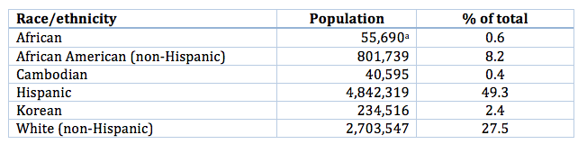
Source: U.S. Census Bureau, 2011-2015 American Community Survey 5-Year Estimates
^a Our study sought to interview individuals who were born in Africa and those with a parent or grandparent born in Africa. This population figure refers only to Africa-born residents, so it underestimates the study’s population of interest.

For this study we used an address-based sample (ABS). ABS offered the most statistically robust approach while containing costs to conduct in-person survey that could collect detailed financial information better than other data collection modes. We used an ABS sample based on the United States Postal Service’s Computerized Delivery Sequence file, which is the best current frame for household surveys in the United States (Harter et al., 2016). Commercial vendors attach flags to the USPS file to indicate household characteristics. One flag indicates the race/ethnicity of the household. Not all households are flagged, the information does not include the date on which the flag was determined, and the accuracy of the information is unknown. Our analysis of the flags for household race/ethnicity found that the accuracy ranged from 6% to 55% depending on the race/ethnicity of interest (Rhodes and Marks, 2018b).To draw the sample, we randomly drew 2,218 households from the USPS list, stratified by major race and ethnic categories—Korean, Cambodian, Hispanic, non-Hispanic black,[1] and other (including unknown). Interviewers visited the address and administered a screener to determine eligibility.We achieved a response rate of 37.4% for the ABS portion of the LA Wealth Inequality study, using the formula for AAPOR response rate 3 (the response rate is 26.1% using AAPOR response rate 1) (AAPOR, 2015).[2] Table 2 shows that more than half of the ABS are in households where we were unable to determine eligibility because no one was ever home, no one ever responded to letters and notes asking them to call us, or no one ever opened the door. Almost 20% are classified as ineligible, meaning they did not match the racial/ethnic categories for this study or they fell into a category whose quota had already been reached.

Table 2. Disposition of Address-Based Sample Cases: LA Wealth Inequality Study

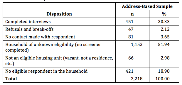
We monitored the sample’s performance to determine whether sampling quotas were met. After completing 451 interviews, the study had successfully reached targets for the African, African American, Hispanic, and white racial/ethnic groups, but would not achieve sufficient numbers of Cambodian and Korean interviews within the available budget. For these two groups, we then transitioned from an address-based sample to a convenience sample.

To locate potential respondents for the convenience sample, we worked with our field interviewers who were from these communities to identify the best ways to contact Cambodian and Korean potential respondents. The field interviewers identified religious institutions, restaurants, and cultural fairs likely to attract Cambodians or Koreans, then visited them and approached adults, explained the purpose of the study, and asked screener questions to see if they were eligible. If yes, interviews were conducted on the spot or scheduled for a convenient time. We completed 25 additional interviews with Cambodian respondents, and 31 additional interviews with Korean respondents.

The Sample and Data Collection: Baltimore

For the Baltimore Incarceration study, the mode of data collection and the target sample size were driven by the amount of available funding, informed by power analyses (available from the authors upon request) and loose estimates about the size of likely financial differences between households that did and did not have a history of incarceration. We found no prior research that could even suggest the magnitude of differences in assets and debts or financial status between households with and without an incarceration history. We targeted completed interviews with approximately 140 nonincarcerated and 140 incarcerated households, with each of those evenly divided between African Americans and whites. Characteristics of the Baltimore City population (Table 3) showed that reaching the white, incarcerated population would be challenging because of their relatively low prevalence in the city.^[3]

Table 3. Estimated Population of Baltimore City Ever Incarcerated, by Race 

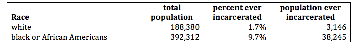
Sources: Population data: U.S. Census Bureau, 2011-2015 American Community Survey 5-Year Estimates. Incarceration data: Bucknor, C. and Barber, A., 2016. “The price we pay: Economic costs of barriers to employment for former prisoners and people convicted of felonies.” CEPR Reports and Issue Briefs 2016-07, Center for Economic and Policy Research, Washington, DC.

Households with a history of incarceration are a hard-to-survey population according to Tourangeau’s criteria. As Table 3 indicates, the incidence of ex-offenders in the general population is low, particularly among the white population of Baltimore City. Ex-offenders tend to be low-income and mobile, making them hard to reach. If an interviewer is able to reach them, they may not want to declare their ex-offender status, making them hard to identify.Because we expected difficulties locating the target populations through strict random digit dialing methods, we took four steps to increase our chances of reaching the population of interest.

1. The sampling frame consisted of only cell phone numbers. A cell-only frame offers nearly full population coverage for the low-income population of interest (Mobile Fact Sheet, 2017). Furthermore, a cell-only frame leads to lower total survey error, eliminates adjustments associated with dual-frame designs, and reduces respondent burden (Peytchev and Neely, 2013).
2. We drew only from cell numbers that were associated with a billing address in Baltimore City or had a number whose area code and first three digits were associated with a Baltimore City rate center. While neither is a perfect indicator of sample member location, the restriction significantly reduced the number of calls (and therefore costs) to reach Baltimore City residents.
3. We removed inactive numbers from the sample frame.
4. We were able to obtain an indicator of household income for some sample frame numbers from commercial vendors and used that to oversample low-income households, who are more likely to have had contact with law enforcement (Rabury and Kopf, 2015).

We drew a final random sample of 43,707 telephone numbers and made 135,163 attempts to call these numbers, administer a screener, and complete an interview with eligible sample members. All working, residential numbers were attempted up to 12 times.

Again using AAPOR response rate 3, we achieved a response rate of 6.7% for the random digit dial sample portion of the Baltimore study (the AAPOR response rate 1 is 6.5%) (see Table 4). This low rate is consistent with typical RDD surveys of the general population. The Pew Research Center (2016) reports that in 2012, the response rate for public opinion polls (not a notoriously difficult telephone survey to conduct) had fallen to 9%.

Table 4: Disposition of RDD Sample Cases: Baltimore Incarceration Study

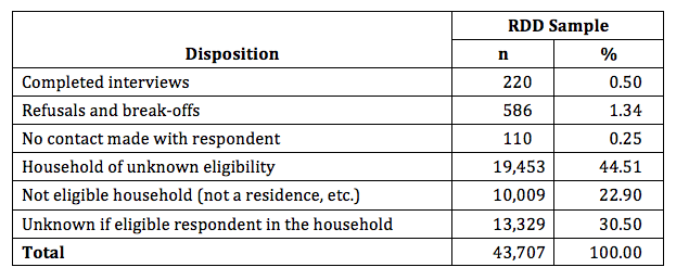
We monitored production rates and used case disposition data to determine how well the sample was performing. Monitoring indicated we would not be able to meet the target number of completed interviews with households that had a history of incarceration, within the amount of resources available.We considered nonprobability options for the sample segment that was falling short and discarded two:

• Snowball sampling would not work because the target population is unlikely to provide information about other ex-offenders. Moreover, the terms of their probation may prohibit them from contacting other ex-offenders (Administrative Office of the U.S. Courts, 2016).
• An intercept survey at or near a prison or jail would require complex and expensive logistical arrangements. We would need to apply to the prisons and receive approval; the sample would consist only of those households with current incarceration, which was not the intent of the study; and it would be costly to visit sufficient numbers of institutions and screen family members for residence in Baltimore City.

A third option was more promising: We devised a low-cost way to increase the sample size by placing a targeted ad to recruit individuals through Facebook and Instagram. The ability to target specific groups is an advantage of social media advertising over other online recruitment methods. Our ad asked users to click on a link to complete a survey if they or someone in their household had been to jail or prison. Once we had developed the ad and Facebook had approved it, Facebook targeted the ad to individuals in Baltimore using data on the user’s reported current residence and the geolocation of the user’s device; we also attempted to target the ad to those with interests that might correlate with our target populations, such as users who had shown an interest in African American history. Facebook does not allow advertisers to target based on certain user characteristics, including race or criminal history.

People who were interested clicked on the link in the ad, answered eligibility questions, and provided contact information. RTI interviewers telephoned those whose answers suggested they met the eligibility criteria and administered a screener. If they were, in fact, eligible and willing to participate, a telephone interview was conducted.

The ad campaign ultimately reached 181,754 social media users, of whom 696 clicked on the ad’s link, completed a few questions on eligibility, and provided a telephone number where they could be reached. We completed 34 interviews with individuals recruited through social media and stopped only (1) after the study’s target for African Americans with an incarceration history had been reached and (2) none of the remaining eligible respondents were whites with an incarceration history, which was the group that needed more respondents (Rhodes and Marks, 2018a).

Results: Los Angeles

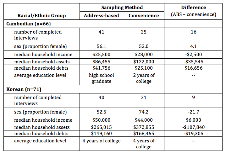
To examine characteristics of respondents from the probability and convenience samples in Los Angeles, Table 5 compares the key demographic characteristics and financial information for Cambodian and Korean respondents. Cambodians are more comparable than Koreans across the two sampling methods for sex and household income; Koreans are more comparable than Cambodians in terms of their average education level.

Table 5. Demographic Characteristics of Probability and Convenience Samples (Cambodian and Korean Respondents)

Results: Baltimore

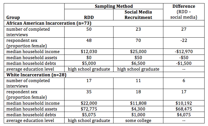
Characteristics of RDD and social media respondents with household incarceration are presented in Table 6. Across the full sample, RDD and social media sample households share similar demographic characteristics (sex, age, education level). Cell sizes for the social media sample are small, but the data show that findings are somewhat inconsistent: for the African American group, social media recruitment resulted in more female respondents and higher income households; for the white group, social media recruitment resulted in respondents with a lower household income yet a slightly higher level of education.

Table 6. Demographic Characteristics of Probability and Nonprobability Samples for Respondents with Household Incarceration History 

Does the Sampling Method Affect the Values of Key Variables?

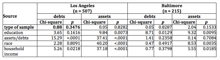
We used convenience and social media samples to increase the number of respondents from low-incidence groups, so the primary methodological question is whether the two types of samples (probability and nonprobability) can be combined for analytical purposes. Because the sample sizes are small, we cannot determine the answer with certainty, but the richness of the data enables us to compare household assets and debts—the primary focus of data collection—across the two types of samples.We use a negative binomial regression model because of its suitability for the nature of the data, particularly that 0 is a valid response to the financial questions that were the focus of the two studies. We estimated Poisson models, but due to the overdispersion of the data, the negative binomial models were more appropriate (Hilbe, 2011). We ran two models—one with assets as the dependent variable, and one with debts as the dependent variable—for the data from the Los Angeles Wealth Inequality study and the data from the Baltimore Incarceration study. In each model, we included the type of the sample—probability or nonprobability—as an independent variable, along with other variables known to be associated with household assets and debts, namely level of education, race, and household income.

Results are provided in Table 7. In sum, the type of sample—probability or nonprobability is not a statistically significant predictor of the dollar amount of household assets or debts. The same results are obtained when computing likelihood ratio statistics for Type 3 analysis, which examines the effect for a variable after all other factors in the model have been accounted for (Table 8).

Table 7. Regression Results to Determine the Effect of Type of Sample on Key Variables of Household Assets and Debts

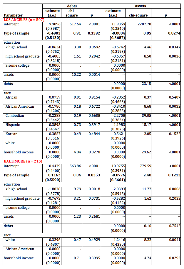
Table 8. Likelihood Ratio Statistics for Type 3 Analysis

We ran a few other models to see if their specification affected the results (data are not presented in this article, but are available from the authors upon request):

• One model added age as an independent variable. It reduced the number of observations in the Baltimore Incarceration study by about one-fourth due to nonresponse. The type of sample remained nonsignificant. We did not include age in the regressions presented in Table 7 to avoid the reduction in sample size.
• Because of the association between the type of sample and respondent race/ethnicity, we ran regressions without the race/ethnicity variable. In the model with assets as the dependent variable, the type of sample became significant. While this result warrants attention, it could be meaningful or it could be due merely to chance given the number of tests we ran.
• Another model added an interaction term for race/ethnicity and type of sample because the nonprobability samples focused on specific racial and ethnic groups. The type of sample remained nonsignificant in these models.
• A third set of models substituted household income for assets and debts as the dependent variable. The type of sample remained nonsignificant in these models.

The preponderance of evidence suggests internal validity when combining probability and nonprobability for analytical purposes with samples of low-incidence populations similar to those studied here.To examine external validity, we have limited options because only limited information is available for the low-incidence populations in our two studies. After considering multiple datasets, we chose to use the U.S. Census Bureau’s 2011-2015, 5-year estimates from the American Community Survey (ACS) from Los Angeles County. Although the ACS does not collect detailed assets and debts information, ACS data do allow us to look at the racial/ethnic groups of interest in our study. The metrics of interest are not absolute dollar comparisons because the groups are not equivalent. Instead, the focus is on the difference from Census data between (1) the probability sample and (2) the combined probability and nonprobability samples. If differences are relatively small, it seems reasonable to combine the two types of samples for analysis.We wanted to perform similar analysis for the Baltimore incarceration study but were unable to locate any data on household income or similar metrics for households with and without a history of incarceration. Thus, we cannot check the external validity of the two types of samples in the Baltimore study.Results for Los Angeles are presented in Table 9. We compared the median income for the two groups in the convenience sample, Cambodians and Koreans. Differences are small: the probability sample versus the combined sample shows a 3.5 percentage point difference for Cambodians and 4.0 percentage points for Koreans. Because the differences are small for these categories, combining the probability and convenience samples for analysis seems to be reasonable.

Table 9: Median Income, Comparisons of Census Data Against Sample Data

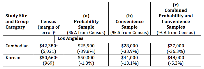
 ^a 2011-2015 American Community Survey, five-year estimate, Table B19013.

Conclusion / Discussion

In this paper, we have expanded the current discourse about nonprobability samples to include those obtained through convenience sampling and through social media recruitment. While Internet panels and respondent-driven methods remain a focus of attention in current survey research literature, consideration of other nonprobability samples is important, particularly when studying groups that are rare in the population. We suggest it may be appropriate to purposefully design studies that rely on a nonprobability sample when locating targeted sample members is so challenging that basic principles underlying probability sampling may be violated.For two distinct studies, we compared key measures for the two types of samples, focusing on respondent demographic characteristics and household financial status. Although our sample sizes are small, the analyses we conducted show that the type of sample was not a significant predictor for the two key variables of interest, namely household assets and debts. Examining the Los Angeles samples against Census data results seems to indicate external validity. Thus, we conclude that the probability and nonprobability samples could be combined within each study to increase the sample size for analytical purposes. We suggest researchers working with probability and non-probability samples for rare populations conduct similar analyses when determining if combining cases from the two types of samples may be appropriate.

[1] In the rest of this document, “black” refers to the African/African American/non-Hispanic category.

[2] AAPOR Response Rate 3 estimates the proportion of eligible cases from those with an unknown eligibility. We used the proportion of eligible cases from all cases of known eligibility for this estimate. AAPOR Response Rate 1, or the minimum response rate, does not include an estimate of the proportion of eligible cases from those with an unknown eligibility.

[3] To determine the percent ever incarcerated, we began with national estimates of the proportion of the US population that had been formerly incarcerated, by race, using US Bureau of Justice Statistics data (Bonczar, 2003). We then applied those proportions to the population of Baltimore City to estimate the number of residents who had ever been incarcerated. Next, we added counts of individuals currently in a Maryland state prison to estimate the number of households with someone currently in state prison. While these estimates are imperfect, they served our goal of getting a general sense of the size of the population of interest to inform planning for data collection.

References

1. Administrative Office of the U.S. Courts. (2016). Overview of probation and supervised release conditions: Chapter 2, Section VIII. Retrieved from http://www.uscourts.gov/services-forms/communicating-interacting-persons-engaged-criminal-activity-felons-probation-supervised-release-conditions
2. American Association for Public Opinion Research. (2015). “Standard Definitions: Final Dispositions of Case Codes and Outcome Rates for Surveys.” https://www.aapor.org/AAPOR_Main/media/publications/Standard-Definitions20169theditionfinal.pdf
3. Ansolabehere, S., and Schaffner, B. F. (2014). Does survey mode still matter? Findings from a 2010 multi-mode comparison. Political Analysis. 22(3), 285-303.
4. Barratt, M.J., et al. (2015). Hidden populations, online purposive sampling, and external validity: Taking off the blindfold. Field Methods, 27(1), 3-21. https://doi.org/10.1177/1525822X14526838
5. Bonczar, T.P. (2003). Prevalence of Imprisonment in the U.S. Population, 1974-2001 (Special Report, NCJ 197976).  Washington, DC:  Bureau of Justice Statistics. Retrieved from: https://www.bjs.gov/content/pub/pdf/piusp01.pdf
6. Boyle, J. M. et al. (2017). Characteristics of the population of internet panel members. Survey Practice, 10(4).  Retrieved from: http://www.surveypractice.org/article/2771-characteristics-of-the-population-of-internet-panel-members
7. Brick, J. M. (2014). Explorations in non-probability sampling using the web. Proceedings of Statistics Canada Symposium 2014. Beyond traditional survey taking:  Adapting to a changing world.  Retrieved from:  https://www.statcan.gc.ca/eng/conferences/symposium2014/program/14252-eng.pdf
8. Davern, M., et al. (2005). The effect of income question design in health surveys on family income, poverty and eligibility estimates. Health Services Research, 40(5P1), 1534–1552.  https://dx.doi.org/10.1111%2Fj.1475-6773.2005.00416.x
9. Harter, R. M., et al. (2016). Address-based sampling. Prepared for AAPOR Council by the Task Force on Address-based Sampling, Operating Under the Auspices of the AAPOR Standards Committee. Oakbrook Terrace, Il.  Retrieved from:  http://www.aapor.org/getattachment/Education-Resources/Reports/AAPOR_Report_1_7_16_CLEAN-COPY-FINAL-(2).pdf.aspx
10. Hilbe, J. M. (2011). Negative Binomial Regression. Cambridge University Press.
11. Kennickell, A. B., et al. (2000). Wealth measurement in the Survey of Consumer Finances: Methodology and directions for future research. Retrieved from http://citeseerx.ist.psu.edu/viewdoc/summary?doi=10.1.1.109.5967
12. Marks, E.L., and Rhodes, B.R. (2017). Wealth inequality in Baltimore: Methodology report. RTI International: Research Triangle Park, NC.
13. Marks, E.L., et al. (2015.) Wealth inequality in Los Angeles: Methodology report. RTI International: Research Triangle Park, NC.
14. Massey, D. (2014). Challenges to surveying immigrants. In R. Tourangeau et al. (Eds.), Hard-to-Survey Populations, pp. 270-292. Cambridge: Cambridge University Press.
15. Mobile Fact Sheet. Retrieved July 26, 2017, from http://www.pewinternet.org/fact-sheet/mobile/
16. Mooi, E., and Sarstedt, M. (2014). A Concise Guide to Market Research: The Process, Data, and Methods Using IBM SPSS Statistics, 2^nd ed. Berlin Heidelberg: Springer-Verlag.
17. Pennay, D.W., et al. (2018). The online panels benchmarking study: A total survey error comparison of findings from probability-based surveys and nonprobability online panel surveys in Australia.  Australian National University: Centre for Social Research and Methods and Social Research Centre Methods Paper. Retrieved from: https://www.srcentre.com.au/our-research/csrm-src-methods-papers/CSRM_MP2_2018_ONLINE_PANELS.pdf
18. Pew Research Center. (2016). “Flashpoints in Polling,” p. 6.
19. Peytchev, A., and Neely, B. (2013). RDD telephone surveys: Toward a single-frame cell-phone design. Public Opinion Quarterly, 77(1), 283–304. https://doi.org/10.1093/poq/nft003
20. Rabury, B., and Kopf, D. (2015). Prisons of poverty: Uncovering the pre-incarceration incomes of the imprisoned. Prison Policy Initiative. Retrieved from https://www.prisonpolicy.org/reports/income.html
21. Rhodes, B.B., and Marks, E.L. (2018a). Using random digit dial and social media recruitment of households impacted by incarceration. Presented at the 73rd Annual Conference of the American Association for Public Opinion Research, Denver, CO.
22. Rhodes, B. B., and Marks, E. L. (2018b). Using ancillary data to identify racial and ethnic subgroups in an address based sample. Presented at the 73^rd Annual Conference of the American Association for Public Opinion Research, Denver, CO.
23. Riphahn, R., and Serfling, O. (2005). Item non-response on income and wealth questions. Empirical Economics, 30(2), 521–538.
24. Tourangeau, R. (2014). Defining hard-to-survey populations. In R. Tourangeau et al. (eds.). Hard-to-Survey Populations, pp. 3-20. Cambridge: Cambridge University Press.
25. Tourangeau, R., et al. (eds.). (2014). Hard-to-Survey Populations. New York: Cambridge University Press.
26. Wang, W., et al. (2015). Forecasting elections with non-representative polls. International Journal of Forecasting, 31(3), 980–991. https://doi.org/10.1016/j.ijforecast.2014.06.001
27. Yeager, D.S., et al. (2011). Comparing the accuracy of RDD telephone surveys and internet surveys conducted with probability and non-probability samples. Public Opinion Quarterly, 75(4), 709–747. https://doi.org/10.1093/poq/nfr020