Using Record Linkage to improve matching rates of subject-generated ID-codes – A practical example from a panel study in schools

---

Abstract

The paper uses data from the first three waves of the German study Health Behavior and Injuries in School Age (GUS) to demonstrate how a record linkage procedure can improve matching rates of subject-generated ID-codes (SGICs) in panel studies. This post-processing technique uses a fuzzy-string-merge to match IDs that do not fit perfectly but are very similar. Other time-constant variables in the dataset were used to verify the matches. With this technique, more than 5 percent of previously unmatched cases could be paired up.

Keywords

Attrition, children, matching, panel data, post-processing, school, self-generated ID-codes, SGIC

Acknowledgement

The GUS study is funded by the German Social Accident Insurance (DGUV).

Introduction

Keeping panel mortality at bay is one of the most important tasks for panel researchers (Kasprzyk et al. 1989, Laurie et al. 1999, Lugtig 2014, Lynn 2018). However, even if respondents participate in all panel waves, there is another challenge, albeit one which has received less attention in methodological literature: Their data also have to be linked correctly in the dataset in order to allow for accurate panel analyses. To give a simple example, imagine a two-year-study with two annual questionnaires. When filling out the survey, there must be some kind of identifier (i. e. the participants’ name, address, e-mail or an ID-code) so that researchers know that the person who filled out the survey in the first year is the same person who completed it in the second year. To successfully achieve this, the identifier must be a) unique and b) persistent over time for every given subject. Both these restraints pose challenges in the fieldwork that do not only vary in their extent from one type of identifier to the other, but also depend on factors such as sample size, time-frame of the study or the social structure of the target population. For example, there may very well be two (or more) people with the same name in a given sample. The bigger the sample, the higher the chances of name duplicates and the longer the timeframe of the study, the higher the chances that people will change their names at some point. Accordingly, participants may change their e-mail- or street address in-between panel waves which could also cause researchers (and statistics software) to believe that they are different people.

Even more potential sources of error are present when identifiers are self-reported instead of assigned as is the case when using subject-generated ID-codes (SGICs). These codes are potentially prone to typing mistakes and memory problems which may also result in erroneously differing (or erroneously matching) codes. However, it can still be feasible to use them, as they allow for completely anonymous data collection. This makes them particularly useful for longitudinal research on sensitive topics or when collecting information from vulnerable populations (Yurek et al. 2008). They also present a feasible strategy when data protection issues are of concern in getting approval for a study from authorities.

SGICs consist of elements inherent and known to the individuals filling out the survey (like one or a few characters of their name, their eye color, their month of birth, etc.). Thus, they can be generated anew by the participants in every wave without having to actually reveal critical personal information. In order to match data from different panel waves properly, two aspects of the makeup of the code are of major importance.

1. Choosing the right length: Longer codes bear a greater risk of errors due to typing mistakes, memory problems and the like (accuracy) while shorter codes are prone to producing duplicates (identifying power) (Direnga et al. 2016). Depending on the size of the sample (or subsample), different lengths are to be preferred.
2. Choosing the right elements: There are many possible elements for the code (see for example Schnell et al. 2010). In theory, any characteristic that is inherent and known to the surveyed individual and that does not change over time is suitable. However, it should also be easy to call upon by the respondents. The most common elements are letters of the father’s and/or mother’s first name.

The German study “Health Behavior and Injuries in School Age (GUS)” is one of these panel surveys that use subject-generated ID-codes (SGICs) to re-identify participants. The students are surveyed in schools over the course of six consecutive annual waves. The goals of this article are to a) assess the severity of ID-errors when working with SGICs and, even more importantly, b) to offer a way to identify and deal with these errors so that researchers can get the most out of their dataset. To achieve this, the GUS study is used as an example. The “data and methods” section offers a detailed description of the target population, sampling procedures and the method of data collection used in the study as well as an overview of the types of matches (correct and false) that can be found in the dataset. Furthermore, the record linkage process used to improve matching rates in the GUS study is described. In the “results” section, it will be shown that the correct application of the record linkage technique can significantly improve data quality. In order to illustrate the concept and processes as simple and clearly as possible, the present paper uses data from the first three panel waves only. However, implications of adding more waves are discussed in the “conclusion/ discussion” section. Additionally, success factors for both the use of SGICs as well as the implementation of record linkage techniques are addressed and potentials for further improvements of linkage algorithms are highlighted. Further information about the study in general as well as results regarding different research questions can, among others, be found in Klocke & Stadtmüller (2018) as well as Stadtmüller et al. (2017).

Data and methods

The data, to which the linking procedures are employed, originate from the German GUS study and include the first three annual waves (N ≈ 10.000 per wave). The target population consists of students in 5^th grade, who were enrolled in German secondary education public schools in the academic year 2014/15. As there is no list of the individual children, the selection was made on the school level. In order to achieve an adequate representation of all federal states in Germany as well as account for the state-specific distribution of school types, a stratified random sample was drawn. The layers in the stratified random sample represent a combination of the federal state, school type, school size and level of urbanity. Some layers, especially those belonging to small federal states, received a higher selection probability, resulting in a disproportionate stratified sample. For pragmatic reasons, all the children in the respective grade of the selected schools were asked to fill out the survey (cluster sampling). Thus, class repeaters from higher grades could enter the sample during the course of the study while students from participating classes who repeated a schoolyear were not surveyed in subsequent panel waves.

The gross sample of the first wave included 854 schools in eleven participating states. Almost a fifth of the schools contacted (17.3 percent) participated in the survey (net sample) amounting to data from 10,621 students in 588 classes and 148 schools. The same classes of the same schools were surveyed again consecutively in grades six and seven. Since primary school in some federal states lasts for six years, schools in these states could only be surveyed from wave 3 (2016/17) onwards and are thus not part of the linkage analyses carried out in this paper. The study could not be carried out in the federal states of Hamburg and Bavaria, as the political bodies (ministries) did not give their consent to the study. Nevertheless, 14 out of 16 federal states in Germany were surveyed in the study.

Data collection

The students were interviewed in their classes within a period of 45 minutes by means of a self-administered questionnaire on a tablet PC (offline classroom survey). In all classes, a trained interviewer was present to introduce the survey, guide students through the generation of the ID-code, offer support in dealing with the tablet PCs and respond to questions concerning the contents of the questionnaire.

Matching

In order for matching via SGICs to work properly, it is important that instructions on how to create them are clear and the elements are free from ambiguity. The SGIC used in the GUS study consists of four elements: 1. The first letter of the student’s own first name, 2. The first letter of the student’s mother’s first name (or the person that comes closest to being their mother), 3. The first letter of the student’s father’s first name (or the person that comes closest to being their father), 4. The month of birth of the respondent. These characteristics should stay constant over time and are easy to recall for the participants (see also Yurek et al. 2008).

To ensure unambiguity, all interviewers received a workshop which included detailed training of the introduction to the survey as well as guiding the participants through the generation of the code. Furthermore, they were also handed out standardized instructions for future reference. Unlike the rest of the survey, which students filled out at their own pace, the whole class did the SGIC-part together and every element of the code was explained to them in detail. This also included mentioning that students who do not know the name of their father or mother should record a “0” instead. However, of the roughly 10,000 students surveyed in each wave, only very few made use of this option (30 in the first wave, 34 in the second, and 36 in the third). In case of doubt about how to correctly fill in the letters, participants could ask the interviewers for guidance. These in turn received a list with frequently asked questions (FAQ) about the survey items (not exclusively but also including the SGIC-items) so that they could give answers in a standardized fashion. Theoretically, a number of scenarios can be imagined in which the students would have trouble choosing the correct letter. For example, they could be unsure if they should use the letters of their parents’ calling names or the names recorded in the passports. Furthermore, they might not know who to count as their father and who as their mother if they have same-sex parents. In practice however, hardly any problems were expressed towards the interviewers regarding these elements.

After each wave, feedback from the interviewers was collected, FAQ lists were updated and procedures adjusted if necessary. For example, in the first two waves, two additional characteristics were surveyed as SGIC-elements. However, eye-color (with “blue”, “grey/green”, and “brown/black” to choose from) and the first letter of the last name of the child’s first teacher in elementary school did not perform well in terms of matching rates. For the first two waves, the longer version of the code only yielded 51 percent matchable cases whereas 67 percent of the cases could be paired up using only the first four elements of the code. Feedback from the interviewers suggests that many children had trouble determining their eye color and/or remembering the name of their first elementary school teacher. Thus, these elements were dropped from the questionnaire from wave 3 onwards and the analyses in this paper only focus on the shorter code.

Once the data was collected, it was prepared for matching. That means, every wave was checked for ID-duplicates within any given school. These duplicates may occur when different students coincidentally generate the same code or when a participant starts over during the interview (for example due to technical difficulties). The duplicates were purged by deleting the case with the higher number of missing answers. When the number of missings was equal, a random selection was made. In total, only around 0.5 percent of the cases in each wave had to be deleted in the process. Afterwards, the remaining 99.5 percent unique cases were checked for their corresponding counterparts in the other waves.  This way, 14,925 completed questionnaires (or 50.1 percent of the overall cases) could be linked across all three panel waves.

Now, finding or not finding a match is one thing, even more important however, is finding the correct matches (and non-matches). These considerations yield four possible outcomes of the matching process between two waves:

1. Correct negative match: The respondent only participated in one of the matched waves and no corresponding code can be found in the respective other wave
2. Correct positive match: The respondent participated in both of the matched waves and the same code can also be found in both waves
3. False negative match: The respondent participated in both of the matched waves but no corresponding code can be found in the respective other wave
4. False positive match: The respondent only participated in one of the matched waves but the same code can still be found in both waves

An approximation of these falsely matched (or falsely unmatched) cases can be achieved by looking at the question: “Have you participated in the study in the last year?” This question was included in the survey program to evaluate if found matches correspond with the answers and we can recommend it as an indicator for the quality of an SGIC.

The consistency of the answers to this question with the matches that can actually be found (and not found) is at 91 percent in wave 2 and 86 percent in wave 3. These cases can be seen as correct matches (outcomes 1. and 2.). As for false matches, 9 percent of the participants in wave 2 (and 12 percent in wave 3) said they had participated in the previous year but no corresponding code could be found in wave 1 (outcome 3.). In terms of false positive matches (outcome 4.), only 0.1 percent (14 participants) had matching codes in wave 1 and 2, although they said they did not participate in the previous year (the same is true for 0.6 percent of the participants in wave 3).

Two conclusions can be drawn from this finding: a) the problem of falsely matched (or unmatched) cases seems to exist but is not a grave one in the GUS study, and b) matching errors are mainly a problem of false negative matches. The goal of the record linkage process is to alleviate this problem whilst not producing more false positive matches. Table 1 gives an example of codes that potentially represents a false negative match to be corrected via record linkage.

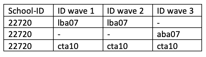
Table 1: Example of data structure before linkage (wide format)

Record Linkage (RL)

The strategy for converting false negative matches to correct positive matches is a fuzzy string-merge. This means that all codes within a school in one wave are matched to the codes of the same school in another wave in a way that small variations in the codes are still counted as matches. This could be accomplished by a simple one-off rule (see Schnell et al. 2010 or Vacek et al. 2017) whereby all cases that do not match perfectly are allowed to vary by one character in order to still count as a match. A more sophisticated approach is to use some kind of algorithm for the fuzzy-matching procedure. This is what was done in the GUS study via the Stata ado “reclink”. The package utilizes a bigram string comparator to accomplish the matching of non-equal yet similar codes. The bigram algorithm splits two strings into all the containing pairs of two consecutive letters (i. e. the word “match” consists of the bigrams “ma”, “at”, “tc”, and “ch”) and compares how many of them they have in common. The matching score is calculated from the total number of coinciding bigrams divided by average number of bigrams in the strings. It ranges from 0 for completely unmatching to 1 for perfectly matching strings (for a detailed description see Churches & Christen 2004). The Stata package also allows for control variables which can either be used to weight the matching score or act as a criterion for exclusion (Blasnik 2010). Thus, this method allows for more granular (and therefore potentially more accurate) results than the one-off rule.

In the GUS study, the year of birth, gender and the number of older siblings are calculated into the matching-score as control variables, while the code of the school has to match perfectly (also referred to as “school linking” by Vacek et al. 2017) from one wave to the other. The threshold of the matching score needed in order for two codes to count as a match was determined by careful calibration. This included an evaluation of the changes in the numbers of correct and false positive and negative cases (as by the question if the students participated in the last year) as well as a manual review of the matched cases. After multiple runs with different configurations, a matching score of 0.85 was chosen as the threshold.

Whenever a non-perfect match is found, the question arises, whether and how to replace the ID-code. This question is crucial given that the codes are also used for linking data in subsequent panel waves. The idea in GUS was that as students get older, they are better able to understand the concept behind the code. Thus, the codes from the earlier wave were replaced with those from the latter. Subsequently, another check for duplicates resulting from the altered codes was implemented. Since the record linkage process can only be carried out between two waves, a total number of three record linkages was necessary to link all the waves to one another. To account for a better understanding of the code over time, the last waves were matched first. The resulting overall process looked as follows:

1. Record linkage wave 3 and 2
   a. Match cases
   b. Overwrite IDs from wave 2
   c. Check for new duplicates
2. Record linkage wave 2 and 1
   a. Match cases
   b. Overwrite IDs from wave 1
   c. Check for new duplicates
3. Record linkage wave 3 and 1
   a. Match cases
   b. Overwrite IDs from wave 1
   c. Check for new duplicates

Figure 1 represents an illustration of this process.

Figure 1: Linkages used for the first three waves of the  GUS study

 

Applying this to the data from table 1, yields the following data structure (table 2).

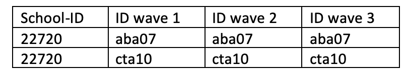
Table 2: Example of data structure after linkage (wide format)

Results

The overall changes in the data structure due to record linkage can be seen in table 3. There are three characters representing the three waves with the value “1” representing a participation in a particular wave.

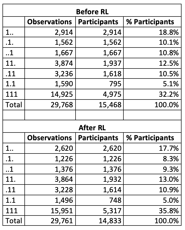
Table 3: Participation rates before and after record linkage (RL)

 

Newly found matches across two waves already allow for better longitudinal analyses. However, panel researchers are often particularly interested in balanced panel data to analyze the full biography of their respondents across all time points (in this case represented as “111”). As shown in table 3, the record linkage procedure increased this number by 342. This is an almost seven percent increase compared to the unlinked dataset. It has to be noted, however, that seven cases had to be omitted due to newly produced ID-duplicates. Thus, there is a bit of a trade-off in terms of total sample size when using this technique.

As noted above, finding more matches is inherent to the process, but the actual goal is finding the correct matches (and non-matches). In order to assess if this was achieved in the GUS study and thus if record linkage is suitable for the use in longitudinal studies, a consistency check was implemented in which participants were asked if they had participated in the study in the previous year. If the answer corresponds to an actual found (or not found) match, the outcome of the matching process can be seen as correct. Table 4 shows the consistency rates for waves 1 and 2 as well as waves 2 and 3. Cases where participants stated “don’t know” are not included in the analysis.

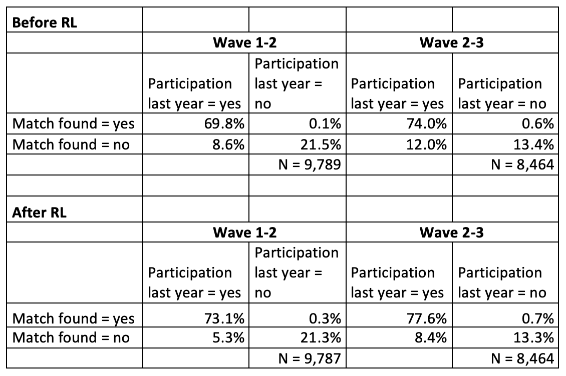
Table 4: Consistency of found matches with the question “Have you participated in the study in the last year?”

 

Even before implementing record linkage, consistency was quite high. In the second wave, 91 percent of the students either stated that they had participated in the previous year and a match was found in the first wave or they said that they had not participated and there was also no matching code. The same is true for 87 percent in the third wave. This is an indicator that overall, the SGICs in the GUS study are an appropriate way to combine data from different waves. Another notable finding is that where discrepancies arose between the statements and the actual matches, it seems to mainly have been a problem of false negative than of false positive matches. There were 8.6 percent suspected false negative matches between waves 1 and 2 and 12 percent between waves 2 and 3 while suspected false positive matches only made up 0.1 percent between waves 1 and 2 and 0.6 percent between waves 2 and 3.

As depicted in table 4, record linkage significantly reduces the number of false negative matches (participation last year = yes, match found = no) while only producing negligible amounts of suspected false positive matches (participation last year = no, match found = yes). This boosts the consistency rate up to 94 percent for waves 1 and 2 and 91 percent for waves 2 and 3. As the original code can be kept in the dataset after record linkage, researchers can even choose to continue using it for those cases that supposedly produce false positive matches. Even if no consistency check like in the GUS study is possible, the present analysis indicates that the outcome of the record linkage process should still be satisfying.

Using the total number of newly linked cases as a measure of the gain from record linkage, an outcome of 1,651 cases (= 5.6 percent of the overall cases) was achieved in the first three waves of the GUS study.

Conclusion/Discussion

There have been a number of publications addressing the use of SGICs for linking longitudinal data across different waves (see for example Damrosch 1986; Dilorio et al. 2000; Galanti et al. 2007; Grube et al. 1989; Kristjansson et al. 2014; Lippe et al. 2019). However, the studies cited in these publications all have much lower overall sample sizes and they do not address and evaluate post-processing techniques to improve matching. The present analyses show that SGICs perform well in the school environment, even if a high number of different schools from diverse regions are surveyed. This holds true regardless of type of school, school size, region or level of urbanity (results of detailed analyses not shown here). Furthermore, record linkage is a suitable way to increase matching rates without a substantial loss in precision.

Crucial prerequisites for a successful implementation of SGICs are a careful choice of characteristics the codes are made up of and an informed decision about the length of the code. This can be quite difficult and even after an extensive review of the literature on SGIC elements, two of the characteristics chosen in the GUS study did not perform well in terms of correct matching. Fortunately, the other four elements still yielded a good degree of uniqueness within the target population. In part, this can be attributed to the fact that the study relies on clustered sampling with every school having its own unique identifier. Thus, the subsamples in which duplicates can occur are relatively small. As even the school with the most surveyed students only had 183 participants (wave 3), chances are low that two students of the same school will incidentally generate the same code. Therefore, a rather short code was suitable for ensuring a sufficient identifying power. For studies with different sample designs and/or bigger (sub-)samples, a longer code is recommended. A possible compromise could be reached by increasing not the number of elements but the number of characters surveyed of these elements (i. e. asking for the first two characters of the mother’s first name instead of just one). This is most likely the approach we will pursue for future studies with SGICs, along with a more careful assessment of the quality of the code in the pretests.

Further factors that can contribute to a correct matching process are clear and unambiguous instructions for the participants as well the use of control variables. The variables can be specifically designed to ask if participants have also participated previously or any variable that is surveyed in every wave and to which the answer should remain constant. The presence of interviewers may also affect the quality of the codes as they can offer support on what to fill in when elements are unknown or unclear to the participant. However, this could not be tested with the data at hand. It should also be noted that asking participants about their previous participation, although seemingly feasible, is not a perfect marker for correct or false matches. To specifically research these dynamics, a study design that lets participants generate their own ID-codes although the real affiliations are known would be desirable.

As for the record linkage, success factors include a careful calibration of the matching score needed to count as a successful match, an informed selection of control variables and a conscious decision about the impact they should have on the matching score. In order to achieve this, repeated manual reviews of the matched cases are recommended. Furthermore, different techniques of fuzzy-matching (as described by Christen & Goiser 2007 for example) could be applied.

One of the biggest challenges associated with using this record linkage technique is the complexity of the linkages in longer running studies. With the algorithms currently available, it is only possible to match two waves at a time. This results in an exponentially growing number of linkages needed to match all the possible wave combinations the more waves are to be matched. For example, only one linkage is needed for matching two waves, whereas four waves require a total number of six linkages (1-2, 2-3, 3-4, 1-3, 2-4 and 1-4). To reduce the number of linkages needed, it may be feasible to only match waves that are no more than two years apart. Furthermore, the order of the linkages can also affect the resulting matches and researchers should evaluate carefully which waves they want to match first. Additionally, they should consider if they want to replace the IDs of the former wave with those of the latter or the other way around.

Hopefully, new algorithms will be developed in the future which are specifically designed for matching SGICs over time and allow for a simultaneous matching of more than two waves. Until then, the existing record linkage possibilities already present a reliable and convenient way to increase matching rates whilst not producing substantial amounts of false positive matches. This can significantly improve the quality of longitudinal analyses.

References

1. Blasnik, M. (2010). RECLINK: Stata module to probabilistically match records. Statistical Software Components.
2. Christen, P., & Goiser, K. (2007). Quality and Complexity Measures for Data Linkage and Deduplication. In F. J. Guillet & H. J. Hamilton (Hrsg.), Quality Measures in Data Mining (S. 127–151). https://doi.org/10.1007/978-3-540-44918-8_6
3. Churches, T., & Christen, P. (2004). Some methods for blindfolded record linkage. BMC Medical Informatics and Decision Making, 4(9). https://doi.org/10.1186/1472-6947-4-9
4. Damrosch, S. P. (1986). Ensuring anonymity by use of subject-generated identification codes. Research in Nursing & Health, 9(1), 61–63. https://doi.org/10.1002/nur.4770090110
5. Dilorio, C., Soet, J. E., Marter, D. V., Woodring, T. M., & Dudley, W. N. (2000). An evaluation of a self-generated identification code. Research in Nursing & Health, 23(2), 167–174. https://doi.org/10.1002/(SICI)1098-240X(200004)23:2<167::AID-NUR9>3.0.CO;2-K
6. Direnga, J., Timmermann, D., Lund, J., & Kautz, C. (2016). Design and Application of Self-Generated Identification Codes (SGICs) for Matching Longitudinal Data. 44th SEFI Conference, 12-15 September 2016, Tampere, Finland.
7. Galanti, M.R., Siliquini, R., Cuomo, L., Melero, J. C., et al. (2007) Testing anonymous link procedures for follow-up of adolescents in a school-based trial: The EU-DAP pilot study. Preventive Medicine 44(2), 174-177. https://doi.org/10.1016/j.ypmed.2006.07.019
8. Grube, J. W., Morgan, M., & Kearney, K. A. (1989). Using self-generated identification codes to match questionnaires in panel studies of adolescent substance use. Addictive Behaviors, 14(2), 159–171. https://doi.org/10.1016/0306-4603(89)90044-0
9. Hsiao, C. (2014). Analysis of Panel Data. Cambridge University Press.
10. Kasprzyk, D., Singh, M. P., Duncan, G., & Kalton, G. (1989). Panel Surveys. New York: John Wiley & Sons Inc.
11. Klocke, A., & Stadtmüller, S. (2018). Social Capital in the Health Development of Children. Child Indicators Research, 1–19. https://doi.org/10.1007/s12187-018-9583-y
12. Kristjansson, A. L., Sigfusdottir, I. D., Sigfusson, J. & Allegrante, J. P. (2014). Self-Generated Identification Codes in Longitudinal Prevention Research with Adolescents: A Pilot Study of Matched and Unmatched Subjects. Prevention Science, 15(2), 205–212. https://doi.org/10.1007/s11121-013-0372-z
13. Laurie, H., Smith, R. A., & Scott, L. (1999). Strategies for reducing nonresponse in a longitudinal panel survey. Journal of Official Statistics, 15, 269–282.
14. Lippe, M., Johnson, B., & Carter, P. (2019). Protecting Student Anonymity in Research Using a Subject-Generated Identification Code. Journal of Professional Nursing, 35(2), 120–123. https://doi.org/10.1016/j.profnurs.2018.09.006
15. Lugtig, P. (2014). Panel attrition: Separating stayers, fast attriters, gradual attriters, and lurkers. Sociological Methods & Research, 43(4), 699–723. https://doi.org/10.1177/0049124113520305
16. Lynn, P. (2018). Tackling Panel Attrition. In D. L. Vannette & J. A. Krosnick (Eds.), The Palgrave Handbook of Survey Research (pp. 143–153). https://doi.org/10.1007/978-3-319-54395-6_19
17. Schnell, R., Bachteler, T., & Reiher, J. (2010). Improving the Use of Self-Generated Identification Codes. Evaluation Review, 34(5), 391–418. https://doi.org/10.1177/0193841X10387576
18. Stadtmüller, S., Klocke, A., Giersiefen, A., & Lipp, R. (2017). Verletzungen auf dem Schulhof – Eine Analyse individueller und kontextueller Faktoren. Das Gesundheitswesen. https://doi.org/10.1055/s-0043-112743
19. Vacek, J., Vonkova, H., & Gabrhelík, R. (2017). A Successful Strategy for Linking Anonymous Data from Students’ and Parents’ Questionnaires Using Self-Generated Identification Codes. Prevention Science, 18(4), 450–458. https://doi.org/10.1007/s11121-017-0772-6
20. Wooldridge, J. M. (2012). Introductory econometrics: A modern approach (5th edition). Nelson Education.
21. Yurek, L. A., Vasey, J., & Sullivan Havens, D. (2008). The Use of Self-Generated Identification Codes in Longitudinal Research. Evaluation Review, 32(5), 435–452. https://doi.org/10.1177/0193841X08316676