Undercoverage of the elderly institutionalized population: The risk of biased estimates and the potentials of weighting

---

Abstract

In most social surveys, the elderly institutionalized population is not part of the target population because it is considered as hard-to-reach and hard-to-interview. The deliberate exclusion of institutionalized elderly from survey samples might cause bias, like previous studies investigating institutionalized elderly persons and their transition to institutions implied. We use a Monte Carlo simulation based on cross-national samples of the Survey of Health, Ageing and Retirement in Europe (SHARE) to test whether the noncoverage and undercoverage of the elderly institutionalized population lead to biased estimates. Moreover, we examined to what extent weights could be used to correct for the underrepresentation of the institutionalized population. Our results show that noncoverage leads to biased estimates in two health-related variables. With respect to undercoverage, the precision of all estimates is better, especially if weights accounting for the hard-to-survey population are applied.

Keywords

coverage bias, Institutionalized population, Monte Carlo Simulation, retirement and nursing homes, SHARE, Survey weighting

Introduction

Large national and cross-national survey programs aim to enable their users in science and the wider public to draw conclusions for the so-called general population, which comprises all residents living in a certain country or region. However, due to practical and financial reasons, surveys usually do not cover the entire population and deliberately exclude certain groups. In round 8, the European Social Survey (ESS) defined its target population as “[a]ll persons aged 15 and over (no upper age limit) resident within private households in each country, regardless of their nationality, citizenship or language” (ESS Sampling Expert Panel 2016, 5). This definition excludes children, the homeless population, and the population living in institutions, such as prisons, retirement and nursing homes, or refugee accommodations. As another example, the Health Survey for England (HSE) “was designed to be representative of the population living in private households in England. Those living in institutions were outside the scope of the survey” (Craig et al. 2015, 13).[1]

The deliberate exclusion of institutionalized residents can be explained with pragmatic reasons on the basis of cost-benefit analyses. Following Tourangeau’s classification of hard-to-survey populations (2014), elderly persons living in institutions can be classified as hard-to-reach and potentially hard-to-interview (Feskens 2009; Schanze 2017). Gatekeepers, such as staff working in institutions or relatives, might prevent interviewers from getting to the respondents because they aim to protect them (see Neuert et al. 2016). Moreover, as the summary of research findings in this paper shows elderly institutionalized residents are more likely to be older and suffer from various non-cognitive and cognitive impairments, which render them more difficult to be interviewed with standard questionnaires (see Sangl et al. 2007).

As long as it can be assumed that excluded parts of the population do not differ to a significant extent from the included survey population, the restricted definition of the target population would not have any negative impact on the generalizability of survey results. This study tests this assumption with regard to the elderly institutionalized population. It is motivated by the following overarching research questions: To avoid coverage bias, do survey programs need to make additional efforts to extend their coverage to the institutionalized population? And secondly, to what extent do survey weights help to counterbalance potential bias due to noncoverage and undercoverage?

Bias in survey results can be driven by two factors: the size of the institutionalized population and the distinctiveness of this population with respect to any variable of interest (Groves et al. 2009; Lessler and Kalsbeek 1992). Regarding the size of the institutionalized population, the latest European census in 2011 counted a cross-national share of 1.3% of institutionalized residents (Eurostat 2015, 45).[2] This proportion gets larger in the age cohorts older than 50 years (1.9%), older than 65 years (3.3%), and in the oldest age cohorts older than 80 years (8.5%).[3] The majority of the institutionalized elderly lives either in health care institutions or retirement and nursing homes (Eurostat 2015). In 2011, this group comprised nearly 2.7 million people and was by far the largest group within the European institutionalized population (ibid.).

As the second factor of coverage bias, the statistical distinctiveness of the institutionalized population comes into play. Moving to a retirement or nursing home implies a strong (self-)selection mechanism. Previous research in the fields of gerontology, medicine, and public health has identified a number of variables that differed significantly between the community-dwelling population living in private households and the institutionalized population (see Section 3). These variables measured socio-demographic, socio-economic, and medical characteristics and are potentially sensitive to coverage bias when institutionalized residents are not covered or undercovered. These differences limit the capacity to make an inference to the whole population, if estimates are based on data that excludes the institutionalized population.

Coverage bias is difficult to quantify, since information about the noncovered population usually is missing (Lessler and Kalsbeek 1992). Our approach uses the data from the Survey of Health, Ageing and Retirement in Europe (SHARE) to run a Monte Carlo simulation. In Europe, SHARE is the only large cross-national survey that has covered the elderly institutionalized population in a comprehensive way (see Schanze 2017). In our simulation, we do not manipulate the statistical distinctiveness of institutionalized residents compared to community-dwelling residents, since this information is contained in the SHARE data. Instead, we alter the coverage rates of institutionalized residents and simulate noncoverage and different degrees of undercoverage. We use the Monte Carlo simulation to detect a possible bias in sample estimates. Moreover, we assess the possibilities and limitations of using survey weights to compensate for the exclusion and inadequate inclusion of the institutionalized population. Our research could be of interest to survey researchers and researchers working with survey data, especially on health or aging.

This paper is structured as follows. In the next section we introduce the concept of coverage bias and also elaborate on the idea of counterbalancing the bias with sample weights. The third section summarizes the previous research on the statistical distinctiveness of the population living in institutions for the elderly. Following this summary, we advance our hypotheses in the fourth section. The fifth section describes the survey data we used and how we processed the data to compile an empirical population for our simulation. In the sixth section, we explain our Monte Carlo simulation approach. This section also describes the weights we applied to the samples. In the seventh section, we present and discuss the results of the Monte Carlo simulation for different conditions of coverage and different weighting schemes. Finally, we draw our conclusion in the last section.

The concept of coverage bias

Analyses of the impact of undercoverage or noncoverage in given survey data are confronted with uncertainty because data on the undercovered parts of the target population is missing by definition (Lessler and Kalsbeek 1992). Very few studies have examined the possible bias if elderly institutionalized respondents are excluded from social surveys. Using a Swedish panel of the population aged 77 years or older, Kelfve and colleagues concluded that limitations in activities of daily living (ADL), restriction of mobility, and psychological problems would be significantly underestimated if 22% of the institutionalized sample units were left out (2013). A Dutch pilot survey of elderly homes and nursing homes found that institutionalized residents had more physical limitations and were in poorer health (Feskens 2009). Since the results were based on a small sample of less than 300 institutionalized respondents, the author concluded cautiously that “excluding residents of elderly and nursing homes may bias survey estimates about the elderly on important population characteristics” (ibid., 95).

The literature on undercoverage mainly covers the issue of frame imperfections, when elements of the target population are excluded from the sampling frame. In the case of institutionalized populations, noncoverage does not arise from frame imperfections. Institutionalized residents are excluded deliberately from most social surveys, which in general leads to biased results. An exclusion from a survey can be organized in two ways. Either the institutionalized residents are cutoff from the sampling frame (see Särndal et al. 1992, 531), or they remain in the sampling frame and are exempt from measurement if sampled. The two procedures have different implications for statistical inference, in particular for the sampling variance, but their estimation bias can be the same. In the following, we only focus on the case of cut-off sampling.

Suppose we have a population of residents who are fully enumerated, so we can create a set of unique indices in which each indice belongs to one element of the population and one element only. This set of indices is our sampling frame, where is the indice associated with the -th person in the population. We denote the set of indices of the institutionalized population as . The set of indices of the non-institutionalized population is then given by .

If our variable of interest is a real valued and positive variable , in cut-off sampling its total for the private population can be estimated by , where is our sample from , i.e , is the observation of variable for the -th element in the frame, and is the probability for including the -th person in the sample from . If we are interest in estimating the total of the entire population , then is biased for if .

To reduce a potential bias, a ratio estimator can be used instead of . If we know the population total of a real valued and positive auxiliary variable , that is also measured in the survey, we are able to construct the following estimator:

where . Estimator is consistent for with . Thus, an approximation to the expected value of is .

The bias of estimator is given by:

and if , if the ratio between auxiliary variable and is the same in the private population and the entire population (see Särndal et al. 1992, 532).

Another class of estimator that could be used to reduce the potential bias of would be the regression estimator. In this case, we use known totals of auxiliary variables, given by , where is the value of the -th auxiliary variable of the -th person in the sampling frame.

We denote the vector of the auxiliary variables for the -th person as .

The general regression estimator for based on can be written as:

where , and is the -th component of the vector of regression coefficients (see Särndal et al. 1992, 225):

If is unbiased for , the regression coefficients of the entire population, then any bias in would be corrected by the second term in .

The regression estimator also can be written as:

where , , and . If we define , we can express as:

where . This expression of the regression estimator highlights its similarity to calibration estimators. With respect to calibration estimators, the so-called design weights, given by , are adjusted by a such that . This adjustment is done so ‘s are as small as possible, while still fulfilling the calibration condition . If as a distance measure between and the chi-square distance is used, the calibration method leads to the regression estimator (see Särndal 2007, 106). Thus, the condition that ensures that is unbiased, i.e., the expected value of is equal to , is the same that ensures that the calibration estimator is unbiased.

Research findings: How do the elderly in institutions differ?

For more than two decades, a growing body of scientific literature in the fields of gerontology and public health have examined the elderly institutionalized population. Various variables have been identified as predictors of transitions from private households to retirement homes and nursing homes. Moreover, comparative analyses of community-dwelling elderly and elderly living in institutions have shown significant differences in various respects. All these studies offer first insights into the statistical distinctiveness of the institutionalized population. The following paragraphs provide a summary of previous research findings. In this section and in Tables 2 and 3 (see Appendix A), we list only the variables that explain institutionalization in multivariate models that control for different confounding variables. If a certain variable explains institutionalization or differs between the community-dwelling population and the institutionalized population, it possibly is subject to coverage bias in social surveys whenever institutionalized residents are excluded from these surveys.

Demographic variables

Demographic and socio-economic variables are very stable, unchanging characteristics of individuals, which is why they belong to the group of predisposing factors for the need of health care (Andersen 1995). They are a first group of strong explanatory factors for the institutionalization of the elderly (see Table 2 for an overview of variables and studies). Across countries and survey designs, nearly all studies found a positive effect of increasing age on institutionalization (e.g., Angelini and Laferrère 2012; Castora-Binkley et al. 2014; Einio et al. 2012; Gaugler et al. 2007; Laferrère et al. 2012; Luppa et al. 2010b; Maxwell et al. 2013; McCann et al. 2012; Rodríguez-Sánchez et al. 2017; Thomeer et al. 2015). The effect of gender on the likelihood of institutionalization is inconclusive in literature. While some studies conclude that female gender increases the likelihood of institutionalization (e.g., Bravell et al. 2009; Kasper et al. 2010; McCann et al. 2012), other studies come to the opposite conclusion, and found a positive effect of male gender (e.g., Gaugler et al. 2007; Luppa et al. 2010b; Martikainen et al. 2009; Pot et al. 2009). The contradictory results can be explained due to the influence of cross-national particularities, different study designs, different times of data collection (see Einio et al. 2012; Himes et al. 2000), and also the strong multicollinearity of gender with other explanatory variables (Einio et al. 2012; Nöel-Miller 2010).

Socio-economic variables

In several studies, socio-economic variables also belong to the group of predisposing factors with significant explanatory power. Residents who own and live in their own houses have a lower probability of moving to institutions for the elderly (e.g., Einio et al. 2012; Gaugler et al. 2007; Luppa et al. 2010b; McCann et al. 2012; Thomeer et al. 2015). Using regional panel data from Sweden, Bravell and colleagues detected a negative correlation between a rising socio-economic status and the likelihood of institutionalization (2009). Some studies have found that both a higher education (Asakawa et al. 2009; Einio et al. 2012) and a higher income (e.g., Angelini and Laferrère 2012; Gaugler et al. 2007; Laferrère et al. 2012; Martikainen et al. 2009; Thomeer et al. 2015 are protective factors against institutionalization. However, two other studies have found the opposite direction of relationship for education and income in other studies. These recent studies using U.S. panel data observed a growing probability of institutionalization with a better education (Castora-Binkley et al. 2014; Thomeer et al. 2015). Concerning income, Rodríguez-Sánchez and colleagues observed a lower probability of institutionalization for individuals with a low household income (2017). Differences at the macro-level with respect to the long-term care system and the care culture could help to explain some of the contradictory results with respect to socioeconomic status (Geerts and Bosch 2012; Laferrère et al. 2012; Suanet et al. 2012).

Social networks and informal care

Marital status and family networks are highly significant independent variables in many studies that aim to explain the institutionalization of the elderly. These variables work as enabling resources, which can protect residents from institutionalization (1995). Indeed, being married protects community-dwelling residents from transition to institutions (e.g., Castora-Binkley et al. 2014; Gaugler et al. 2007; Luppa et al. 2010b; Rodríguez-Sánchez et al. 2017) compared to larger odds of institutionalization for residents who are not married (e.g., Asakawa et al. 2009; Bravell et al. 2009; Thomeer et al. 2015), widowed (Angelini and Laferrère 2012; Einio et al. 2012; Nöel-Miller 2010; Thomeer et al. 2015), or divorced (Thomeer et al. 2015). As a consequence, living alone (e.g., Gaugler et al. 2007; McCann et al. 2012; Pimouguet et al. 2016) without a partner in the household (Désesquelles and Brouard 2003; Laferrère et al. 2012) increases the likelihood of institutionalization, whereas co-residence with a partner and/or children decreases the likelihood of institutionalization (Angelini and Laferrère 2012; Kasper et al. 2010; McCann et al. 2012; Rodríguez-Sánchez et al. 2017; Thomeer et al. 2015). Apart from a partner, some studies also observed a negative effect of having (grand-)children (e.g., Kasper et al. 2010; Nöel-Miller 2010; Rodríguez-Sánchez et al. 2017) on institutionalization. Marital status and family networks, as well as additional social networks are closely linked to availability of informal care in private households. Smaller social networks (Hays et al. 2003; Luppa et al. 2010b; Maxwell et al. 2013) increased the probability of institutionalization.

Health-related variables

Health-related variables are strong predictors of institutionalization across all kinds of study designs within different countries (see Table 3 for an overview of significant explanatory variables). First, cognitive impairments (e.g., Castora-Binkley et al. 2014; Einio et al. 2012; Gaugler et al. 2007; Luppa et al. 2010b; Maxwell et al. 2013; Rodríguez-Sánchez et al. 2017; Thomeer et al. 2015; Toot et al. 2017) increase the probability that community-dwelling residents have to move to institutions for the elderly, for example, due to the prevalence of dementia (e.g., Einio et al. 2012; Laferrère et al. 2012; Luppa et al. 2010b; Nihtilä et al. 2008; Toot et al. 2017. In addition to dementia, a number of medical conditions, especially if they occur simultaneously, also are associated with a higher likelihood of institutionalization (e.g., Angelini and Laferrère 2012; Einio et al. 2012; Gaugler et al. 2007; Luppa et al. 2010b; Maxwell et al. 2013; Rodríguez-Sánchez et al. 2017; Toot et al. 2017). Turning from the objective measures of health to a measurement of subjective health, a bad self-rated health also increases the likelihood of institutionalization according to some studies (Castora-Binkley et al. 2014; Einio et al. 2012; Hancock et al. 2002; Luppa et al. 2010b; McCann et al. 2012; Nöel-Miller 2010).

Autonomy and mobility

Often, following a critical state of health, an elderly person’s ability to cope with autonomous daily living is diminished. With respect to the likelihood of institutionalization, studies have found a positive influence of so-called limiting long-term illnesses (Grundy and Jitlal 2007; McCann et al. 2012), functional impairments (Luppa et al. 2010b; Maxwell et al. 2013; Pot et al. 2009), mobility difficulties (Hays et al. 2003; Thomeer et al. 2015; Toot et al. 2017; Von Bonsdorff et al. 2006), motor limitations (Angelini and Laferrère 2012), and physical dependency (Désesquelles and Brouard 2003). Closely related to the concept of physical dependency, many studies have examined limitations in basic activities of daily living (ADL) and instrumental activities of daily living (IADL). ADL includes limitations in walking, dressing, eating, bathing, going to the toilet, and getting in and out of bed. IADL measures limitations with respect to managing money, preparing meals, getting groceries, using the telephone, and taking medications. Studies have found that both ADL (e.g., Bravell et al. 2009; Gaugler et al. 2007; Laferrère et al. 2012; Rodríguez-Sánchez et al. 2017; Thomeer et al. 2015; Toot et al. 2017) and IADL (e.g., Castora-Binkley et al. 2014; Laferrère et al. 2012; Thomeer et al. 2015; Toot et al. 2017) often are very strong predictors of institutionalization.

Previous research suffers from two limitations. First, many studies relied on regional data in the absence of national data (see Agüero-Torres et al. 2001; Bravell et al. 2009; Hancock et al. 2002; Hays et al. 2003; Maxwell et al. 2013; Pimouguet et al. 2016; Riedel-Heller et al. 2000; Von Bonsdorff et al. 2006). Second, analyses are more difficult to carry out due to the very small number of institutionalized residents. The small number of respondents might also serve as an explanation for some of the contradictory results.

Our study contributes to the current research by testing the impact of noncoverage and undercoverage with a larger dataset of institutionalized respondents. Moreover, we distinguish different degrees of undercoverage and also assess whether survey weights can counterbalance a potential coverage bias. To our knowledge, it is the first simulation analysis of the bias caused by the exclusion of the elderly institutionalized population in social surveys.

Hypotheses

Following from the previous section, the hard-to-survey population living in institutions for the elderly differs in many respects from their community-dwelling counterparts. They have a worse objective and subjective state of health and are more often suffering from cognitive and functional impairments. They are older, have a different marital status, and have lived alone more frequently prior to institutionalization. Considering the statistical distinctiveness of the institutionalized population described in the previous section, it is our overarching hypothesis that bias arises when institutionalized respondents are excluded from the sample. We tested two different variables because bias affects different variables to a different extent. On the basis of the literature, we chose two health-related variables.

If institutionalized residents are not covered adequately in survey samples, we expect an underestimation of a variable measuring the limitations in ADL. This underestimation is expected to have a significant impact on the estimated mean and on the estimated share of respondents without limitations in ADL. For our second dependent variable, self-rated health, we assume an overestimation of the mean in our samples compared to the overall empirical population. The share of respondents with poor self-rated health is assumed to be underestimated.

The bias might be reduced by applying calibration weights when analyzing the sample data drawn from sampling frames with noncoverage or undercoverage, as described in Section 2. Kelfve and colleagues weighted the samples without institutionalized respondents for age and gender, and concluded that the weighting did not improve the estimation substantially since the bias persisted (2013). We also tested whether weights for age and gender improve the point estimates of samples that suffer from noncoverage and undercoverage. In addition to traditional survey weights, we tested weights calibrated on age, gender, and institutionalization. Those weights can be used by surveys that try to cover the hard-to-survey population living in institutions but might suffer from undercoverage. In case of noncoverage, the latter weights cannot be used. When no institutionalized respondents are in the sample, it is not possible to calibrate on the variable measuring institutionalization.

For both types of weights, we expect a decreasing bias. We assume that the marginal positive effect of the survey weights calibrated on age and gender will be much smaller than that for the extended survey weights, which also account for the undercovered population. Our focus for the analysis is on the interplay of weights with an decreasing undercoverage of institutionalized respondents. We assume that weights cannot fully eliminate the bias under the condition of noncoverage, but they will yield better results with an increasing coverage rate.

Data

For our simulation-based analysis, we used data from the Survey of Health, Ageing and Retirement in Europe (SHARE) to construct an empirical population, from which we can select samples for our simulation study. SHARE is a cross-national panel survey, which collects its data in the face-to-face mode and uses strict quality standards and a harmonization across the participating countries preceding the data collection (Börsch-Supan et al. 2013). Moreover, to our best knowledge, SHARE is the only cross-national social survey that includes institutionalized respondents to a significant extent.

With the exception of the third wave, we used all six waves of SHARE data collected in a number of European countries and Israel, approximately every 2 years between 2004 and 2015 (Börsch-Supan 2017a,b,c,d,e). In the first wave in 2004, the SHARE target population was defined as all households with “at least one member born in 1954 or earlier, speaking the official language of the country and not living abroad or in an institution such as a prison during the duration of field work” (Klevmarken et al. 2005, 30). However, in addition to this minimum definition of the target population, residents of institutions for the elderly also are officially part of the SHARE target population and shall be sampled and interviewed if possible (De Luca et al. 2015; Klevmarken et al. 2005; Lynn et al. 2013). SHARE also uses proxy interviews (Börsch-Supan et al. 2013), which is especially important with respect to hard-to-interview groups like institutionalized residents.

Before describing our methods, we need to mention one limitation of the data we used. According to the documentation of SHARE, institutionalized residents suffer from undercoverage. A number of countries reported in their sampling design forms that it was not possible to sample institutionalized respondents in the first wave and in refreshment samples because they were excluded from the sampling frames (De Luca et al. 2015; Klevmarken et al. 2005; Lynn et al. 2013). In the first wave, this was the case in Austria, France, Greece, Italy, and Switzerland (Klevmarken et al. 2005). In contrast, an equal number of countries reported that their target population included institutionalized residents in the first wave (ibid.).[4] Due to these frame imperfections, the first group of countries does not cover the entire institutionalized population, since it includes only the community-dwelling respondents who moved to institutions between two survey waves. As a consequence, the sample of institutionalized respondents suffers from undercoverage and could be biased.[5] However, even within those countries that reported a noncoverage of institutionalized residents in the baseline wave we identified institutionalized respondents (Table 4 in the Appendix).[6] Nevertheless, the undercoverage diminishes the potential to generalize our simulation results and our conclusions are restricted to our empirical population.

Given the small share of institutionalized respondents in the separate waves, we cumulated five of the six waves of SHARE and only excluded the third wave of the panel because its content differs largely from all the other waves.[7] For every panel respondent, we only retained the most recent interview in our dataset. However, if a respondent lived in an institution and moved back to a private household in a subsequent wave, we dropped the more recent interview conducted in the private household.[8] We included every respondent who was interviewed between 2004 and 2015 by SHARE with only one observation in our dataset. Moreover, in the pooled dataset we dropped six countries with less than 50 interviews in institutions[9] , but still cover most parts of Europe and Israel (see Table 4 in the Appendix B) We also dropped all respondents younger than 50 years at the point of data collection. These respondents are only eligible as a partner of a SHARE respondent and are not a representative sample of the population younger than 50 years.

In total, we obtained a dataset with 100,595 observations, among these 2,514 nursing home interviews, which amounted to 2.5% of our empirical population. Due to missing values in some of the variables we used in our analysis, we dropped another 1,929 cases (1.9% of the pooled sample) and obtained our final empirical population of 98,666 cases, among these 2.47% institutionalized residents ( = 2,441).

A comparison of the cases without any item nonresponse in the variables of interest with the dropped cases shows that item nonresponse occurs more often in interviews with institutionalized respondents (3.8% of the excluded respondents and therefore a higher share than in the empirical population). Moreover, the excluded population is older than the included population (69.3 years compared to 67.9 years), is more often widowed (19% compared to 15.7% of the included units), has more limitations in activities of daily living (0.67 compared to 0.46), and feels less healthy (2.66 compared to 2.81). Very small differences between included and excluded respondents occur in terms of income, the number of children, and education. In addition, the two populations do not differ significantly in the distribution of gender.

Variables of interest

Since we used several waves of a panel survey in a cross-sectional analysis, we had to make sure that all the variables we used in our analysis have been measured in the same way for all the five waves (see Appendix B for the main variables). To assess the statistical impact of an exclusion of institutionalized residents, we analyzed two different variables that have been salient for the institutionalized population in previous research: an index of the limitations in activities of daily living (ADL) and self-rated health.

Our first variable of interest measures the dependency of respondents and evaluates their ability to run a household and cope with daily living. Respondents were provided with a showcard that listed various activities of daily living (ADL). They answered which activities they could not execute because of “a physical, mental, emotional or memory problem.” For our analysis, we used six items classified by SHARE as ADL items and created a 9-level additive index with three additional dummy variables that belong to the group of items that measure the limitations in instrumental activities of daily living (IADL). These nine items displayed a high tau-equivalent reliability (Cronbach’s = 0.89) and loaded clearly on a single factor in an exploratory factor analysis. Our first dependent variable is a count variable with a very large number of respondents with an outcome of 0 (zero-inflated, see Table 1).

As our second variable of interest we analyzed self-rated health. This variable measured the subjective health of respondents, which implicitly encompasses physical and mental health. SHARE used the U.S. version of this variable to measure self-rated health on a 5-level scale in all five waves.

Institutionalization

To operationalize long-term institutionalization, we relied on three different variables to generate a dummy variable that captured whether a respondent lived in a private household or in an institution during the interview. Since the second wave, SHARE interviewers registered whether a sampled address was a private household or a nursing home when they arrived at the address. According to the SHARE codebook[10] , a nursing home “provides all of the following services for its residents: dispensing of medication, available 24-hour personal assistance and supervision (not necessarily a nurse), and room & meals”.[11] In addition to this process-generated variable, we also coded all the respondents as institutionalized residents, who reported to have lived permanently in an institution during the last year.[12] As a third variable, we used the type of building in which a respondent lives. If respondents either answered this question with category 7 “a housing complex with services for elderly” or 8 “special housing for elderly (24 hours attention)“, we coded these cases as being institutionalized.[13]

Monte Carlo Simulation

In this section, we describe our simulation-based analytical approach with the different coverage conditions and weights that we applied in the Monte Carlo simulation.

To evaluate the bias of the different estimation strategies of different coverage scenarios of the institutionalized population, we repeatedly selected samples from our empirical population. The sampling design of the simulations study is a stratified sample, in which the 15 countries in our empirical population serve as the strata. Within the strata, we selected individuals using a simple random sample. The sampling fraction is 3% and the allocation of the sample size is done proportionally to the number of persons within the strata. Thus, all persons in the sampling frame have an almost equal inclusion probability of 0.03 (i.e., ignoring the rounding problem of the actual allocation).

We considered five different coverage scenarios, and we constructed five different sampling frames to include 0%, 25%, 50%, 75%, and 100% of the institutionalized population. Thus, as our sampling frames were , with , where  is a simple random sample from with sampling fraction . To construct  , is portioned into four disjoint random subsets, each of size . , with . From each of the five sampling frames, we selected 1000 samples with the sampling design described above. In the following, we denote as the coverage rate of the institutionalized population in the sampling frame.

Estimators

Our statistics of interest are the (1) mean of limitations in ADL, (2) the share of respondents without any limitations in ADL, (3) the mean of self-rated health, and (4) the share of respondents with poor self-rated health.  To estimate these statistics, we employed three different estimators. The first estimator is:

where is a sample from frame , is the design weight given by , and is the measurement or category indicator for one of the variables of interest for the -th person in the sampling frame.

For our second estimator, we used a regression estimator as described in Section 2 to estimate the total of our variable of interest, which we divided by the sum of the regression estimator or calibration weights. Thus, we produced the following estimator:

where , and is constructed as described in Section 2. Like many other social surveys, SHARE uses mainly region, age, and gender as auxiliary variables for constructing cross-sectional calibration weights at the level of individuals (De Luca et al. 2015). For , we also used age in 5 categories and gender and their known totals over all element in frame as auxiliary variables. This estimation strategy reflects the situation where a survey with non or partial coverage of the institutionalized population uses aggregate data for weighting purposes, that covered the entire population including institutionalized residents (e.g., census data).

For our third estimator , we added institutionalization to the survey weights described above. By weighting for the hard-to-survey domain that suffers from undercoverage, we aim to examine whether this approach is a feasible option for surveys to counterbalance their insufficient coverage. However, this approach does not work for survey samples without any institutionalized residents.

For each of the 1,000 samples from each of the five coverage scenarios, we estimated for our two variables of interest the proportions and the overall mean using all three estimators described in Section 6. Additionally, we calculated the 95% confidence intervals (CI) of all the point estimates for each of the samples. The confidence intervals are constructed as follows:

where is any of our point estimates under consideration and is its variance estimate. The confidence intervals enabled us to check whether the deviations between a sample estimate and the true share or true mean in our empirical population were significant enough to be defined as biased. Every confidence interval that missed the true value was marked as rejected. If there was no bias at all, the expected proportion of rejected samples would be 5%.

Results

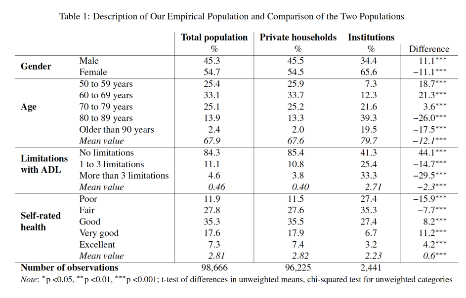
Table 1 provides a description of our empirical population for some variables, and compares the institutionalized respondents and the community-dwelling respondents. The table reveals considerable differences between the two domains. In our empirical population, more women than men live in institutions, whereas the community-dwelling population is more gender balanced. The institutionalized population is more than 12 years older on average.

Concerning the two dependent variables, nearly 60% of all institutionalized respondents have at least one or more limitations in activities of daily living, compared to a significantly lower share of 14.6% in private households. As a consequence, the mean values of the ADL variable differ significantly between the two populations. Regarding the second dependent variable, more respondents in institutions reported a poor or fair state of health compared to the community-dwelling population. Only 10% of all institutionalized respondents rated their health as very good or excellent. The aggregate differences in the mean value of self-rated health are less distinct compared to the ADL variable, although they are still statistically significant.

The first column of Table 1 provides the values of the variables of our total empirical population, which includes community-dwelling and institutionalized respondents. A comparison of this column with the second column depicting the aggregate values for the community-dwelling population already shows the impact of coverage bias in the case of noncoverage of the institutionalized population. Only slight differences occur in terms of gender distribution and the number of children. The community-dwelling population definitely deviates from the true values with respect to other variables. The joint share of the two oldest age cohorts differs by one percentage point. Regarding the two dependent variables, only the variable measuring limitations in ADL seems to be significantly biased. Adding the institutionalized respondents to the community-dwelling respondents decreases the share of people without any limitations in ADL from 85.4% to 84.3%. The differences in reports of self-rated health are less diverging if the community-dwelling population is compared with the total population. The results of Table 1 can be interpreted as a census of our empirical population. The following analyzes show how survey samples perform, if they do not cover institutionalized residents at all or cover them insufficiently.

Noncoverage

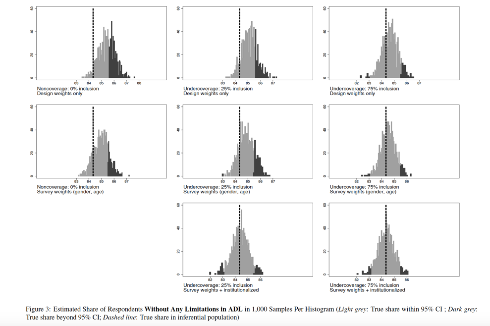
Figure 1 and Table 6 (see Appendix C) provide the results of the simulation for limitations in ADL. Each box plot in Figure 1 contains the relative bias of estimates in 1,000 samples with the given coverage condition and the given weighting scheme compared. The relative bias is computed as the ratio of the estimate and the true value and expressed in percentage in this case. Table 6 provides the mean values from those 1,000 samples and the share of samples that were rejected on the basis of their confidence intervals. In the case of noncoverage, nearly two thirds of all samples failed to predict the true mean of the ADL variable for our empirical population. The estimation of the share of respondents without any limitations in ADL is less sensitive to bias. The simulation replicated the differences shown in Table 1, since the samples missed the true value (84.34%) by about one percentage point on average. As a result, 41.4% of the samples missed the true share with their confidence intervals. The graphical analysis in Figure 3 shows that these 414 samples estimated a share of respondents without limitations in ADL to be between 85.6% to 87.6%.

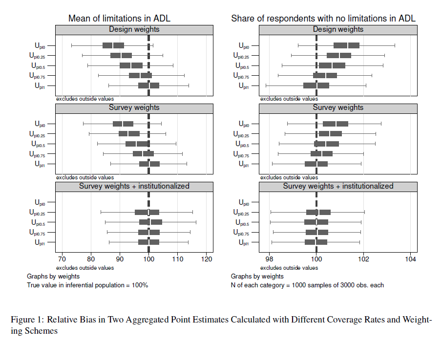
In line with our hypothesis, using estimator improved the precision under the condition of noncoverage (), but could not eliminate the bias entirely. Both boxes move closer to the dashed lines that indicate the true values. As it can be seen in Table 6, using age and gender as auxiliary variables reduced the number of estimates for the mean of ADL whose CIs did not include the true mean of 42.3%. Regarding the estimated share of respondents without limitations in ADL, only 21.6% of all CIs did not include the true value. As pointed out in Section 6, the estimator , which adds institutionalization to the survey weights, cannot be applied under the condition of noncoverage, since the domain of institutionalized respondents is empty.

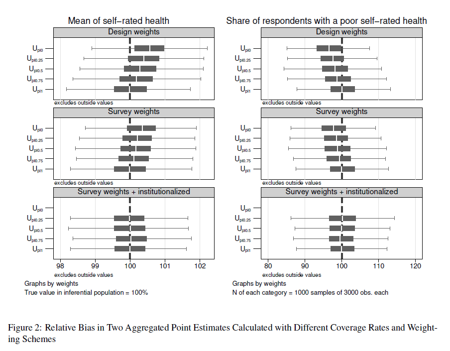
ADL is a relatively strong predictor of institutionalization and should be biased with a higher likelihood than other variables as a consequence. According to Table 1, self-rated health is less different between the community-dwelling population and the overall population. Indeed, our simulation confirms that the bias in estimates related to self-rated health is weaker than in those for ADL. The design-weighted estimator overestimated the average self-rated health and underestimated the share of persons with poor self-rated health (see Figure 2). However, the estimations are closer to the true values than for ADL. 10.9% and 11.5% of all CI estimates using missed the true share of poor self-rated health and the true mean of self-rated health, respectively (see Table 7). Although still displays bias for the statistics of ADL, it made a substantial difference in the measurement of self-rated health. Using decreased the number of CI estimates that did not include the true share of poor self-rated health to 6.4%.

The results underline the varying impact of bias on two different health-related variables and point estimates. With respect to the ADL variable, the estimation of the mean was more prone to bias than the estimation of the share of respondents without any limitations in ADL. With respect to self-rated health, the estimation of the share of poor self-rated health and the prediction of the mean were equally sensitive to bias. This finding can be explained also by the different scales of the two variables. ADL is a count variable with a 9-level scale and many respondents with a zero value. Every third institutionalized respondent reached a value larger than 3 on the ADL scale (see Table 1), and this group drove the true mean upwards. The self-rated health variable has a 5-level scale, and smaller values indicating poor self-rated health were more prevalent among the institutionalized respondents. As a consequence, the true mean is less affected by the group of institutionalized respondents.

Undercoverage

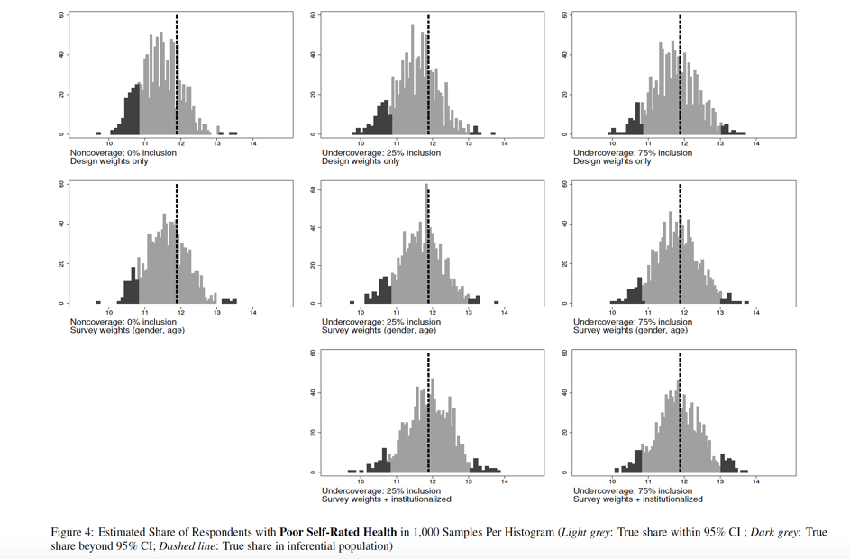
Following the scenario of noncoverage using the sampling frame , we increased the proportion of the institutionalized population that we included in the sampling frame in four steps. The scenarios , , and can be described as sampling frames with undercoverage. For the three frames 18 (), 37 (), and 55 () institutionalized persons were expected to be part of the samples. Figures 1 and 2 show the percentage deviation of estimates for each undercoverage scenario, the respective Tables in Appendix C provide the share of CI estimates that did not include the true value. Figures 3 and 4 present the distribution of all sample estimates for different undercoverage scenarios, for the estimators for the share of respondents without any limitations in ADL and the share of individuals with poor self-rated health, respectively (see Appendix C for the respective Figures for the remaining coverage conditions).

As we assumed, the bias in the ADL variable becomes smaller with an increasing coverage of the institutionalized population (see Figure 1). Using , an expected 18 institutionalized individuals in a sample of nearly 3,000 respondents made a difference and decreased the CI noncoverage rate to 43.6% of all samples. The precision of and got even better. Figure 3 shows how the distributions of estimates were shifted to the left, bringing their center closer to the true value. As with noncoverage, using auxiliary information for estimation decreased the likelihood of bias in all the undercoverage frames. reduced the CI noncoverage rate of the share of respondents without limitations in ADL by about 50% compared to (see second row in Figure 3). The extended survey weights resulted in nearly unbiased samples from onward. Only 6.0% of all samples missed the true value with their confidence interval, and 6.8% of all samples missed the true mean with their CI when survey weights accounted for the undercovered group. For the traditional survey weights (), the CI noncoverage rates approached the 5% threshold for (see Table 6).

Regarding self-rated health, the bias in the case of noncoverage was smaller than for the ADL variable. This observation also holds for the different scenarios of undercoverage. With an increasing , the bias in is reduced in both point estimates. The slight overestimation of the mean of self-rated health and the underestimation of the share of respondents with poor self-rated health were progressively corrected. This is in line with our expectations. In addition, most of the weighted estimators of self-rated health were estimated almost without any bias of an of at least 0.5 (Table 7). Weighting with age, gender and institutionalization as auxiliary variables produced almost unbiased estimates in every scenario of undercoverage (see Figure 2 and last row of Figure 4).

The results for promote the overall conclusion that conventional survey weights might indeed help to counterbalance the bias in health-related variables. In the case of undercoverage, the few institutionalized residents received larger weights because they were older and more often female than the average respondent. The weights significantly improved the precision of the estimates compared to simple design-weights. This improvement can only be achieved if institutionalized residents are included in the population statistics used for weighting. For instance, the Health Survey for England excludes institutionalized residents from the population statistics used for calibrating their weights (Craig et al. 2015, 25) and misses the chance to counterbalance the impact of noncoverage at least indirectly. In addition to traditional survey weights, weighting directly for the hard-to-survey group proves to be even more efficient in our simulation. The estimator yielded unbiased results for all scenarios of undercoverage. However, one drawback of this method is the necessity to have at least some respondents from the hard-to-survey population in the sample.

Conclusion

The present study quantified the bias caused by the noncoverage or undercoverage of the population living in institutions for the elderly and tested whether survey weights can help to counterbalance the bias. Given the very small share of institutionalized respondents, we pooled the panel data of the Survey of Health, Ageing and Retirement in Europe (SHARE). We obtained a dataset of nearly 100,000 respondents, among them more than 2,400 institutionalized respondents. Taking this data as the basis for our simulation, we randomly sampled 5,000 samples of 3,000 observations with different coverage rates of institutionalized respondents. For each of the 5,000 samples, we calculated descriptive statistics and applied three different types of weights.

The simulation results prove that coverage bias affects variables to a different extent and even influences different kinds of point estimates in different ways. A variable measuring the limitations in activities of daily living (ADL) is heavily biased if respondents living in institutions are excluded from the samples. Our second variable measuring the self-rated health of respondents also was biased, but the impact of noncoverage is less pronounced. All other things being equal, the precision of all the point estimates improved with an increasing coverage rate. We tested three conditions of undercoverage and found a clear pattern of a decreasing coverage bias when more institutionalized residents were included.

Weighting the samples for age and gender improved all the point estimates in the case of noncoverage or undercoverage. If survey researchers make sure that the population margins they use for weighting include institutionalized residents, they can improve the precision of their estimates even without including the elderly institutionalized population in their survey. The likelihood of unbiased results gets even better if institutionalized residents are included in the samples, even if this domain suffers from undercoverage. Undercoverage also allows researchers to weight for the hard-to-survey population as such, if population statistics on their size and relevant characteristics are available. In our simulation, the extended survey weights eliminated bias for both health-related variables. This shows the high potential of calibrating the weights on the size of undercovered populations to reduce bias.

Our simulation-based analysis has a number of limitations. By analyzing the respondents of SHARE with a simulation-based approach, we wanted to arrive at some general conclusions about the risk of biased estimates in social surveys. One advantage of our simulation is that it does not rely on synthetic observations, but considers real respondents instead. Especially in the case of an understudied group like institutionalized populations, a simulation with synthetic observations would require a large number of assumptions and thus raise many question about the validity of simulation results.

Nevertheless, our conclusions only hold true for the empirical population we compiled. The potential to generalize our results beyond the simulation depends on the data quality and the validity of our methods. As we mentioned previously, some of the SHARE countries reported undercoverage of institutionalized respondents in the first wave and refreshment waves (De Luca et al. 2015; Klevmarken et al. 2005; Lynn et al. 2013). Panel attrition due to non-contact and refusals is a second major factor that could lead to a biased longitudinal sample of institutionalized respondents. Moving to an institution constitutes an external shock that probably increases the likelihood of non-contact and/or refusal (see Lugtig 2014).[14] Due to undercoverage and panel attrition, our empirical population certainly misses institutionalized residents in the general population, although the share of these respondents in our simulation (2.5%) is close to the share of institutionalized residents in the overall population older than 50 years (1.9% according to the European census).

Regarding our method, the data we used was collected during a period of 11 years between 2004 and 2015. We considered this data as cross-sectional data, and thus, might have missed the changes of contextual factors that could influence our results as confounding variables. In this study, we only analyzed a limited number of two variables. Both variables are health-related variables, and therefore, they have a higher likelihood of being biased with respect to the noncoverage or undercoverage of the elderly institutionalized population. We suggest taking our results of the ADL variable as the maximum effect coverage bias can have on survey estimates. We assume that the results for our second variable shows a more common influence of coverage bias. The presentation of research findings in Section 3 puts forward more variables that could be biased and should be tested, such as marital status, family composition, objective health, and socio-economic status.

A lot of research remains to be done on the institutionalized population. We only analyzed mean values and the distribution of variables. It is easier to interpret bias in descriptive statistics, but since they are only the starting point of most scientific papers, it would be very informative to extend the analysis to cover inferential statistics as well. For instance, the bias of regression coefficients could be tested by comparing the predicted outcomes of an equation with the respective results obtained in samples with equal coverage. Our study focused on the question of whether it is necessary to include institutionalized residents. Future research should examine whether it is also feasible to include this domain.

Our results could have implications for survey research in Europe because most social surveys in Europe deliberately exclude the institutionalized population, since it is considered as hard-to-survey (see Tourangeau 2014). Within our study, we asked whether survey programs need to make additional efforts to extend their coverage to the institutionalized population. Our results show for two health-related variables that surveys of an aging population indeed risk to obtain biased survey estimates if the institutionalized population is excluded. Moreover, the results suggest to abstain from the strategy to exclude institutionalized residents, because of the concern to cover this population insufficiently. Undercoverage is less sensitive to bias than noncoverage, especially when a sample is weighted for age and gender or even for institutionalization itself.

---

Endnotes

[1] See Schnell for a description of excluded groups in German surveys (1991).

[2] This figure also contains a small number of homeless residents. Excluding them from the Eurostat data with the publicly available census hub tool does not change the overall share of 1.3% (see Eurostat 2016).

[3] Own calculations using the census hub homepage (Eurostat 2016). We used the category “Occupants living in a collective living quarter” of a variable measuring housing arrangements (HC39).

[4] Denmark, Germany, Netherlands, Spain, and Sweden

[5] As a matter of fact the panel will be representative of the institutionalized population in the very long run, at the moment when the population does not include any institutionalized citizens that have been institutionalized before the first wave of the panel was recruited (Lynn 2011). This assumption only holds true if the panel survey does not draw any biased refreshment samples in the meantime, and if panel attrition does not lead to a stronger decrease of panel members from the institutionalized populations.

[6] See also De Luca et al. for a similar observation of a mismatch of country reports about noncoverage and the de facto presence of nursing home residents in the SHARE data (2015: 78).

[7] SHARELIFE collected retrospectively information on life events of the SHARE respondents (see Börsch-Supan and Schröder 2011). Some variables used in this analysis were not part of the questionnaire in SHARELIFE.

[8] This rule only affected a small number of 508 respondents, adding up to 0.2% of the entire pooled sample before dropping duplicate observations across waves.

[9] Croatia, Hungary, Ireland, Poland, Portugal, and Slovenia

[10] Generic CAPI coverscreen, can be downloaded at http://www.share-project.org/data-documentation/questionnaires.html

[11] 1,424 institutionalized respondents were identified as institutionalized residents by the interviewers in our final empirical population.

[12] We added 326 respondents to the group of institutionalized residents based on their reply to this variable. These respondents were classified as community-dwelling respondents by the interviewers. From the second wave onward, respondents were usually not asked this question if interviewers identified their place of living as an institution.

[13] Additional 691 respondents were classified as institutionalized according to their replies to this questions.

[14] Please note, empirical evidence about the effect of institutionalization on panel membership is lacking to our best knowledge.

---

Appendices

Appendix A: Variables explaining institutionalization

Appendix B: Data and variables

Appendix C: Additional results

References

1. Agüero-Torres, Hedda, Eva Von Strauss, Matti Viitanen, Bengt Winblad, and Laura Fratiglioni (2001). “Institutionalization in the elderly: The role of chronic diseases and dementia. Cross-sectional and longitudinal data from a population-based study”. Journal of Clinical Epidemiology 54(8): 795–801.
2. Andersen, Ronald (1995). “Revisiting the Behavioral Model and Access to Medical Care: Does it Matter?” Journal of Health and Social Behavior 36(1): 1–10.
3. Angelini, Viola and Anne Laferrère (2012). “Residential mobility of the European elderly”. CESifo Economic Studies 58(3): 544–569.
4. Asakawa, Keiko, David Feeny, Ambikaipakan Senthilselvan, Jeffrey Johnson, and Darryl Rolfson (2009). “Do the determinants of health differ between people living in the community and in institutions?” Social Science and Medicine 69(3): 345–353.
5. Börsch-Supan, Axel (2017a). Survey of Health, Ageing and Retirement in Europe (SHARE) Wave 1. Data Release: 6.0.0. SHARE-ERIC. DOI: 10.6103/SHARE.w1.600.
6. Börsch-Supan, Axel (2017b). Survey of Health, Ageing and Retirement in Europe (SHARE) Wave 2. Data Release: 6.0.0. SHARE-ERIC. DOI: 10.6103/SHARE.w2.600.
7. Börsch-Supan, Axel (2017c). Survey of Health, Ageing and Retirement in Europe (SHARE) Wave 4. Data Release: 6.0.0. SHARE-ERIC. DOI: 10.6103/SHARE.w4.600.
8. Börsch-Supan, Axel (2017d). Survey of Health, Ageing and Retirement in Europe (SHARE) Wave 5. Data Release: 6.0.0. SHARE-ERIC. DOI: 10.6103/SHARE.w5.600.
9. Börsch-Supan, Axel (2017e). Survey of Health, Ageing and Retirement in Europe (SHARE) Wave 6. Data Release: 6.0.0. SHARE-ERIC. DOI: 10.6103/SHARE.w6.600.
10. Börsch-Supan, Axel, Martina Brandt, Christian Hunkler, Thorsten Kneip, Julie Korbmacher, Frederic Malter, Barbara Schaan, Stephanie Stuck, and Sabrina Zuber (2013). “Data Resource Profile: The Survey of Health, Ageing and Retirement in Europe (SHARE)”. International Journal of Epidemiology 42(4): 992–1001.
11. Börsch-Supan, Axel and Mathis Schröder (2011). “Retrospective Data Collection in the Survey of Health, Ageing and Retirement in Europe”. In: SHARELIFE Methodology. Ed. by Mathis Schröder. Mannheim Research Institute for the Economics of Ageing (MEA): 5–10.
12. Bravell, Marie, Stig Berg, Bo Malmberg, and Gerdt Sundström (2009). “Sooner or later? A study of institutionalization in late life”. Aging Clinical & Experimental Research 21(4-5): 329–337.
13. Castora-Binkley, Melissa, Hongdao Meng, and Kathryn Hyer (2014). “Predictors of long-term nursing home placement under competing risk: Evidence from the health and retirement study”. Journal of the American Geriatrics Society 62(5): 913–918.
14. Craig, Rachel, Jennifer Mindell, and Vasant Hirani (2015). Health Survey for England: Methods and documentation. Vol. 2. Leeds (UK): Health and Social Care Information Centre Health.
15. De Luca, Giuseppe, Claudio Rossetto, and Frederic Malter (2015). “Sample design and weighting strategies in SHARE Wave 5”. In: SHARE Wave 5: Innovations & Methodology. Munich: MEA, Max Planck Institute for Social Law and Social Policy: 75–84.
16. Désesquelles, Aline and Nicolas Brouard (2003). “The Family Networks of People aged 60 and over Living at Home or in an Institution”. Population 58(2): 201–227.
17. Einio, Elina, Christine Guilbault, Pekka Martikainen, and Michel Poulain (2012). “Gender Differences in Care Home Use Among Older Finns and Belgians”. Population 67(1): 75–101.
18. ESS Sampling Expert Panel (2016). “Sampling Guidelines: Principles and Implementation for the European Social Survey”. London: ESS ERIC Headquarters.
19. Eurostat (2015). “People in the EU: who are we and how do we live? 2015.” Publications Office of the European Union, Luxembourg.
20. Eurostat (2016). European Statistical System – Census Hub. URL: https://ec.europa.eu/CensusHub2.
21. Feskens, Remco (2009). “Difficult Groups in Survey Research and the Development of Tailor-made Approach Strategies”. PhD thesis. Universiteit Utrecht.
22. Gaugler, Joseph, Sue Duval, Keith Anderson, and Robert Kane (2007). “Predicting nursing home admission in the U.S: a meta-analysis”. BMC Geriatrics 7(13): 1–14.
23. Geerts, Joanna and Karel van den Bosch (2012). “Transitions in formal and informal care utilisation amongst older Europeans: The impact of national contexts”. European Journal of Ageing 9(1): 27–37.
24. Groves, Robert, Floyd Fowler, Mick Couper, James Lepkowski, Eleanor Singer, and Roger Tourangeau (2009). Survey Methodology. Second edi. New York: John Wiley & Sons, Inc.
25. Grundy, Emily and Mark Jitlal (2007). “Socio-demographic variations in moves to institutional care 1991-2001: A record linkage study from England and Wales”. Age and Ageing 36(4): 424–430.
26. Hancock, Ruth, Anthony Arthur, Carol Jagger, and Ruth Matthews (2002). “The effect of older people’s economic resources on care home entry under the United Kingdom’s long-term care financing system”. Journals of Gerontology, Series B 57(5): 285–293.
27. Hays, Judith, Carl Pieper, and Jama Purser (2003). “Competing risk of household expansion or institutionalization in late life.” Journals of Gerontology, Series B 58(1): S11–S20.
28. Himes, Christine, Gert Wagner, Douglas Wolf, Hakan Aykan, and Deborah Dougherty (2000). “Nursing home entry in Germany and the United States”. Journal of Cross-Cultural Gerontology 15(2): 99–118.
29. Kasper, Judith, Liliana Pezzin, and J. Bradford Rice (2010). “Stability and changes in living arrangements: Relationship to nursing home admission and timing of placement”. Journals of Gerontology, Series B 65 B(6): 783–791.
30. Kelfve, Susanne, Mats Thorslund, and Carin Lennartsson (2013). “Sampling and non-response bias on health-outcomes in surveys of the oldest old”. European Journal of Ageing 10(3): 237–245.
31. Klevmarken, Anders, Bengt Swensson, and Patrik Hesselius (2005). “The SHARE Sampling Procedures and Calibrated Design Weights”. In: The Survey of Health, Ageing and Retirement in Europe – Methodology. Ed. by Axel Börsch-Supan and Hendrik Jürges. September. Chap. 5: 28–37.
32. Laferrère, Anne, Aaron Van Den Heede, and Karel Van Den Bosch (2012). “Entry into institutional care: predictors and alternatives”. In: Active ageing and solidarity between generations in Europe. Ed. By Axel Börsch-Supan, Martina Brandt, Howard Litwin, and Guglielmo Weber: 253–264.
33. Lessler, Judith T. and William D. Kalsbeek (1992). Nonsampling Error in Surveys. New York: John Wiley & Sons, Inc.
34. Lugtig, Peter (2014). “Panel attrition: separating stayers, fast attriters, gradual attriters, and lurkers”. Sociological Methods & Research 43(4): 699–723.
35. Lumley, Thomas (2004). “Analysis of Complex Survey Samples”. Journal of Statistical Software 9(1). R package verson 2.2: 1–19.
36. Lumley, Thomas (2010). Complex surveys: a guide to analysis using R. Wiley series in survey methodology. Hoboken, N.J: John Wiley.
37. Lumley, Thomas (2016). survey: analysis of complex survey samples. R package version 3.32.
38. Luppa, Melanie, Tobias Luck, Elmar Brähler, Hans Helmut König, and Steffi G. Riedel-Heller (2008). “Prediction of institutionalisation in dementia: A systematic review”. Dementia and Geriatric Cognitive Disorders 26(1): 65–78.
39. Luppa, Melanie, Tobias Luck, Herbert Matschinger, Hans-Helmut König, and Steffi Riedel-Heller (2010a). “Predictors of nursing home admission of individuals without a dementia diagnosis before admission – results from the Leipzig Longitudinal Study of the Aged (LEILA 75+).” BMC health services research 10: 186.
40. Luppa, Melanie, Tobias Luck, SiegfriedWeyerer, Hans Helmut König, Elmar Brähler, and Steffi Riedel-Heller (2010b). “Prediction of institutionalization in the elderly. A systematic review”. Age and Ageing 39(1): 31–38.
41. Lynn, Peter (2011). “Maintaining Cross-Sectional Representativeness in a Longitudinal General Population Survey”. Understanding Society Working Paper Series, 2011 – 04.
42. Lynn, Peter, Giuseppe De Luca, Matthias Ganninger, and Sabine Häder (2013). “Sample Design in SHARE Wave Four”. In: SHARE Wave 4 Innovations & Methodology. Ed. by Frederic Malter and Axel Börsch-Supan. München: MEA, Max Planck Institute for Social Law and Social Policy: 74–123.
43. Martikainen, Pekka, Heta Moustgaard, Michael Murphy, Elina Einiö, Seppo Koskinen, Tuija Martelin, and Anja Noro (2009). “Gender, Living Arrangements, and Social Circumstances as Determinants of Entry into and Exit from Long-Term Institutional Care at Older Ages: A 6-Year Follow-Up Study of Older Finns”. Gerontologist 49(1): 34–45.
44. Maxwell, Colleen, Andrea Soo, David Hogan, Walter Wodchis, Erin Gilbart, Joseph Amuah, Misha Eliasziw, Brad Hagen, and Laurel Strain (2013). “Predictors of Nursing Home Placement from Assisted Living Settings in Canada”. Canadian Journal on Aging 32(04): 333–348.
45. McCann, Mark, Emily Grundy, and Dermot O’Reilly (2012). “Why is housing tenure associated with a lower risk of admission to a nursing or residential home?Wealth, health and the incentive to keep ’my home’”. Journal of Epidemiology & Community Health 66(2): 166–169.
46. Neuert, Cornelia, Otto Wanda, Angelika Stiegler, Clara Beitz, Robin Schmidt, Katharina Meitinger, and Natalja Menold (2016). “SHARE Gatekeeper-Project: Cognitive Pretest”. GESIS-Projektbericht, 2016/07: Mannheim.
47. Nihtilä, Elina, Pekka Martikainen, Seppo Koskinen, Antti Reunanen, Anja Noro, and Unto Häkkinen (2008). “Chronic conditions and the risk of long-term institutionalization among older people”. European Journal of Public Health 18(1): 77–84.
48. Nöel-Miller, Claire (2010). “Spousal Loss, Children, and the Risk of Nursing Home Admission”. Journals of Gerontology, Series B 65(3): 370–380.
49. Pimouguet, Clément, Debora Rizzuto, Pär Schön, Behnaz Shakersain, Sara Angleman, Marten Lagergren, Laura Fratiglioni, and Weili Xu (2016). “Impact of living alone on institutionalization and mortality: A population-based longitudinal study”. European Journal of Public Health 26(1): 182–187.
50. Pot, Anne Margriet, France Portrait, Geraldine Visser, Martine Puts, Marjolein Broese van Groenou, and Dorly J H Deeg (2009). “Utilization of acute and long-term care in the last year of life: comparison with survivors in a population-based study”. BMC Health Services Research 9(1): 139.
51. R Core Team (2017). R: A Language and Environment for Statistical Computing. R Foundation for Statistical Computing. Vienna, Austria. URL: https://www.R-project.org/.
52. Riedel-Heller, Steffi G, Astrid Schork, Herbert Matschinger, and Matthias C Angermeyer (2000). “Recruitment procedures and their impact on the prevalence of dementia: Results from the Leipzig Longitudinal Study of the Aged (LEILA75+)”. Neuroepidemiology 19(3): 130–140.
53. Rodríguez-Sánchez, Beatriz, Viola Angelini, Talitha Feenstra, and Rob Alessie (2017). “Diabetes-Associated Factors as Predictors of Nursing Home Admission and Costs in the Elderly Across Europe”. Journal of the American Medical Directors Association 18(1): 74–82.
54. Sangl, Judith  et    (2007).  “The  Development  of  a  CAHPSR©Instrument  for  Nursing  Home  Resi-dents (NHCAHPS)”.Journal of Aging & Social Policy19(2): 63–82.
55. Särndal, Carl-Erik (2007). “The calibration approach in survey theory and practice”. Survey Methodology 33(2): 99–119.
56. Särndal, Carl-Erik, Bengt Swensson, and Jan Wretman (1992). Model Assisted Survey Sampling. New York: Springer-Verlag.
57. Schanze, Jan-Lucas (2017). “Report on sampling practices for the institutionalized population in social”. Deliverable 2.16 of the SERISS project funded under the European Union’s Horizon 2020 research and innovation programme (GA No: 654221). URL: www.seriss.eu/resources/deliverables.
58. Schnell, Rainer (1991). “Wer ist das Volk? Zur faktischen Grundgesamtheit bei „allgemeinen Bevöllkerungsfragen”: Undercoverage, Schwererreichbare und Nichtbefragbare”. Kölner Zeitschrft für Soziologie und Sozialpsychologie 1(43): 106–137.
59. Suanet, Bianca, Marjolein Broese van Groenou, and Theo van Tilburg (2012). “Informal and formal home-care use among older adults in Europe: can cross-national differences be explained by societal context and composition?” Ageing and Society 32(03): 491–515.
60. Thomeer, Mieke Beth, Stipica Mudrazija, and Jacqueline Angel (2015). “How do race and hispanic ethnicity affect nursing home admission? Evidence from the health and retirement study”. Journals of Gerontology, Series B 70(4): 628–638.
61. Toot, Sandeep, Tom Swinson, Mike Devine, David Challis, and Martin Orrell (2017). “Causes of nursing home placement for older people with dementia: a systematic review and meta-analysis”. International Psychogeriatrics 29(02): 195–208.
62. Tourangeau, Roger (2014). “Defining hard-to-survey populations”. In: Hard-to-Survey Populations. Ed. by Roger Tourangeau, Brad Edwards, Timothy Johnson, Kirk Wolter, and Nancy Bates. Cambridge University Press: 3–20.
63. Von Bonsdorff, Mikaela, Taina Rantanen, Pia Laukkanen, Timo Suutama, and Eino Heikkinen (2006). “Mobility limitations and cognitive deficits as predictors of institutionalization among communitydwelling older people”. Gerontology 52(6): 359–365.