Using Geospatial Data to Monitor and Optimize Face-to-Face Fieldwork

---

Abstract

Interviewers occupy a key position in face-to-face interviews. Their behavior decisively contributes to the quality of surveys. However, monitoring interviewers in face-to-face surveys is much more challenging than in telephone surveys. It is often up to the interviewer when they conduct the interviews and which addresses they work on first. Nevertheless, homogeneous fieldwork, i.e. that which has a geographically similar processing status, is particularly essential for time- and event-dependent studies such as election studies. Irregular fieldwork combined with geographical differences can have substantial impacts on data quality. Using the example of the German Longitudinal Election Study (GLES), we propose and present a visual strategy by plotting key indicators of fieldwork onto a geographical map to monitor and optimize the fieldwork in face-to-face interviews. The geographic visualization of fieldwork can be an additional tool not only for election studies, but also other studies.

Keywords

face-to-face, fieldwork monitoring, geographical visualization, interviewer observation, survey management

1. Introduction

Contemporary face-to-face surveys face great challenges: survey costs are rising, response rates continue to fall and therefore the potential for nonresponse bias is increasing (Beullens et al. 2018; Groves and Couper 1998; de Leeuw et al. 2018; Groves, Williams and Brick 2018). Thus, accurate fieldwork monitoring is becoming more and more important. Although fieldwork monitoring aims to improve the quality of the survey while accounting for costs (Edwards et al. 2017: 255), the discovery of irregularities does not always lead directly to interventions. The decision-making process often involves a variety of actors (principal investigators, agency, survey manager), which requires presenting the results as intuitively and clearly as possible so that they are comprehensible to others. Therefore, effective fieldwork monitoring should consider quality control as well as its essential communication function.

For this purpose, there are already numerous methods and procedures to accompany, document, and adjust fieldwork (Edwards et al. 2017; Mohadjer and Edwards 2018; Groves and Heeringa 2006; Kreuter et al. 2010; several contributions in this volume). Many methods are based on the calculation of key performance indicators (KPIs) and figures, which record and evaluate the current status, process, and progress of the fieldwork and possibly also offer forecasts for future data collection (Beullens et al. 2018; Rogers et al. 2004; Schouten et al. 2011; Williams and Brick 2018). Even though these classic methods are appropriate for monitoring fieldwork, many of these methods do not take into account the geographical aspects of fieldwork (Malter 2013; several contributions in this volume).

However, geographical asymmetries in fieldwork – i.e. processing considerably more addresses in specific geographic regions – is a major concern in the fieldwork monitoring of election surveys. Therefore, visual, map-based tools can be an additional way to capture the fieldwork progression in another dimension (quality control); at the same time, they are an excellent way to communicate problems in fieldwork more effectively to decision-makers (communication function). Based on these findings, the field agencies and principal investigators could collaborate on an intervention to immediately counteract the imbalance. Efficient and straightforward solutions could be, for example, the retraining of interviewers or the reinforcement of problematic regions with additional interviewers.

This article extends the toolbox of fieldwork monitoring by presenting spatial visualization strategies. Data from the fieldwork monitoring of the 2017 German Longitudinal Election Study (GLES) are used (Bieber and Bytzek 2013; Schmitt-Beck et al. 2010), which is a well-suited example because of its short field period and the deep concern about regionally uniform progress in fieldwork (Roßteutscher et al. 2019).

First, we briefly review the challenges in fieldwork monitoring and specifically focus on the requirements of election surveys. We then discuss the possibilities that geospatial data offers in terms of optimizing fieldwork. Thereafter, we describe the current state of fieldwork monitoring in the GLES cross-sectional study before moving on to our geographic visualization tool. In the last section, we discuss our visualization method and illustrate the various opportunities that this tool offers for monitoring and optimizing fieldwork based on the 2017 GLES cross-sectional study. We close the article with a discussion of both the challenges and advantages of the geographic visualization of fieldwork monitoring.

2. The Challenges of Fieldwork Monitoring, with a Special Focus on the Requirements of Election Surveys

Interviewers hold a crucial position in face-to-face surveys (Ackermann-Pick 2018; Jäckle et al. 2013; Loosveldt 2008; Meier Jæger 2016; Schaeffer et al. 2010). Although the principal investigators, survey manager, and field agencies plan the interviews and fieldwork in great detail and establish concrete guidelines on how to conduct the interviews, the interviewer ultimately contacts the respondents and conducts the interviews on their own. In organizing their actual work, the interviewers have leeway, as long as they follow certain rules (e.g. frequency and quantity of contact attempts, contact at different times of the day) (Roßteutscher et al. 2019). The interviewers are thus allocated a powerful position. A further problem is that many interviewers work on a freelance basis and are thus often involved in multiple projects, possibly for several agencies simultaneously, and/or hold the interviews as a part-time job. All of this impacts their work schedule and makes monitoring, adjusting, and assessing fieldwork difficult.

Election studies provide an additional challenge because of their time-sensitive nature. The GLES cross-sectional study, for example, consists of two separate surveys with two independent samples: the pre- and post-election cross-sections (Roßteutscher et al. 2019). The pre-election survey starts eight weeks prior to the federal election. An earlier field start is not feasible, since the study aims to capture citizens’ electoral behavior as close as possible to Election Day. The election study then ends on the day before the federal elections. The end cannot be postponed under any circumstances, as the questionnaire is particularly geared to the time before the federal elections. In order to conduct appropriate analyses, the number of cases must be completed by this time. On the day after the federal elections, the post-election survey is sent into the field. The goal here is to interview as many citizens as possible in the first weeks after the election so as to minimize the time between the interview and the focused event – the federal election – although an extension of the field period is, in principle, possible. However, this is undesirable for quality reasons.

A second important factor in election surveys is related to time sensitivity: the need for homogeneous field development. Ideally, this means that regional differences in fieldwork progress are non-existent or compensated for and that the processing status in all areas is comparable. In addition to the known problem of nonresponse, this need is driven by two other factors. First, voting behavior differs according to region; generally speaking, the eastern part of Germany votes differently than the western part, while the southern part votes differently than the northern part. To guarantee the quality of the study, it is essential to obtain comparable rates of contact, cooperation, and response across the country. Identifying problematic regions early makes it possible to intervene sooner. Second, election studies aim to obtain information about the actual voting behavior on the day of the election. As it is impossible to conduct face-to-face surveys on Election Day itself, the data collection phase must be extended. However, the risk potentially exists that respondents change their election behavior as a result of election campaigns or (political) events (e.g. environmental catastrophes, political parties or individual politicians’ behavior) during this field period, which can produce measurement errors. Events often have a strong regional nature that is somehow linked to local politics and only changes the electoral behavior of certain regional groups. To minimize this type of measurement error, it is crucial to develop a standardized field that is temporally and regionally homogeneous.

The problems with the interviewers described above and the time-sensitivity of election studies necessitate very close and detailed supervision of the fieldwork. This should also include the geographical dimension of fieldwork, which helps to identify irregularities, structural problems, and problematic regions as well as enable principal investigators to provide the agencies with valid evidence of difficulties in fieldwork. In an ideal scenario, poor-performing interviewers could then be replaced or particularly good interviewers could be sent to problematic areas.

3. Fieldwork Monitoring and the Use of Geospatial Data

Increasing digitalization with computer-assisted interviewing and data processing enables stakeholders to collect and monitor process data (i.e. paradata) in real-time during the field period (Biemer 2010). Paradata collection has significantly improved the quality of fieldwork monitoring in regards to process evaluation, monitoring, and management in the last several years (Kreuter et al. 2010: 282). Following Edwards et al. (2017: 255), “making well-informed tradeoffs to reduce error while the data are still being collected is often better than estimating (and living with) the error afterward.”

Numerous methods and tools have been developed to check the quality of surveys, many of which are currently being used as standard forms of quality control by well-known institutes and organizations, such as Statistics Canada, the US Census Bureau, the Institute of Social Research at the University of Michigan, and Statistics Sweden (Kreuter et al. 2010). Examples of widespread and established systems include Continuous Quality Improvement (CQI) (Biemer 2010; Biemer and Caspar 1994; Morganstein and Marker 1997), Computer-Assisted Recorded Interviewing (CARI) (Biemer 2010; Hicks et al. 2010; Mitchell et al. 2008; Thissen 2014; Thissen and Myers 2016) and the Field Supervisor Dashboard from Westat (Edwards et al. 2017). The idea underlying each of these methods originates from the field of industrial product optimization and compares current processes with general processes; when deviations occur, stakeholders can discuss adequate actions and, if necessary, intervene (Kreuter et al. 2010). CQI and Westat’s system are quality management tools, which transform paradata from the field into graphics and key performance indicators (Biemer 2010; Edwards et al. 2017).

Some of these tools also use Geographic Information Systems (GIS) or the Global Positioning System (GPS). Geographic data can improve the planning, observing, and monitoring of interviewers’ behavior (Edwards et al. 2017: 256; Nusser 2007; Thissen et al. 2016; Vercruyssen and Loosveldt 2017; Wagner et al. 2017). Currently, geolocation information primarily helps to increase the efficiency of data collectors by analyzing routes (Olson and Wagner 2013) or identifying falsifications of interviews (Eckman 2014; Olson and Wagner 2013; Vercruyssen and Loosveldt 2017). Edwards et al. (2017: 266) attribute enormous benefit, especially in regards to the latter, in the 2015 federal election, and report “how falsification detection can be dramatically improved in speed, level of effort, and coverage with GIS tools. They provide a quick, inexpensive way to detect falsified interviews across 100% of the sample”. In 2003, Westat implemented a similar approach called EAGLE (Efficiency Analysis through Geospatial Location Evaluation) that collects geocoordinates via the interviewer’s login on the laptop and smartphones, which make it possible to geographically measure key events, interviewer travel routes, and interviewer activity (Edwards et al. 2017). Despite this potential, the number of publications and the usability of geographic data are thus far limited (Thissen et al. 2016).

While some studies have already used geospatial data to monitor fieldwork, they largely focused on monitoring the individual interviewers and their travel patterns. However, geospatial data is also helpful for cartographically displaying the field development on a more abstract level. Such maps could be useful tools, especially for time- and event-dependent studies like election surveys, which are subject to the problems described above. This can enable more intuitive field control and simplifies the identification of problematic areas. Finally, geographic visualization can also comprehensibly communicate existing field problems to the decision-maker, thus reinforcing decisions. Using this approach does not even require the GIS or GPS data of the interviewer. In the first step, address data and status reports suffice.

4. Fieldwork Monitoring of GLES – Data and Current Status

In the GLES cross-sectional study fieldwork progress is monitored weekly based on status reports/contact protocols compiled by the interviewers. Thereby, it is important to note that the GLES cross-section is an interviewer-based study with a registered sample, in which frame information about the persons to be interviewed is available in advance. For each target person, information exists on the disposition code of the last contact attempt in a respective week, the number of contact attempts, the interviewer number, the sample point number, the federal state, the date, and sociodemographic information like sex and age. The following analyses are based on data from the GLES post-election cross-section (Roßteutscher et al. 2019).

Currently, the fieldwork is monitored and checked by several key indicators that can be aggregated on different levels (sample level, interviewer level, sampling point level, federal state level):

(1) Total number of interviews / Proportion of interviews conducted on the gross

(2) Contact attempts: Proportion of contacted households on gross

(3) Finalized cases: Proportion of finally processed cases on gross

Further parameters are calculated to assess the quality of the fieldwork, such as response rate, cooperation rate, and refusal rate.

Figure 1: Indicators of the Current Fieldwork Monitoring

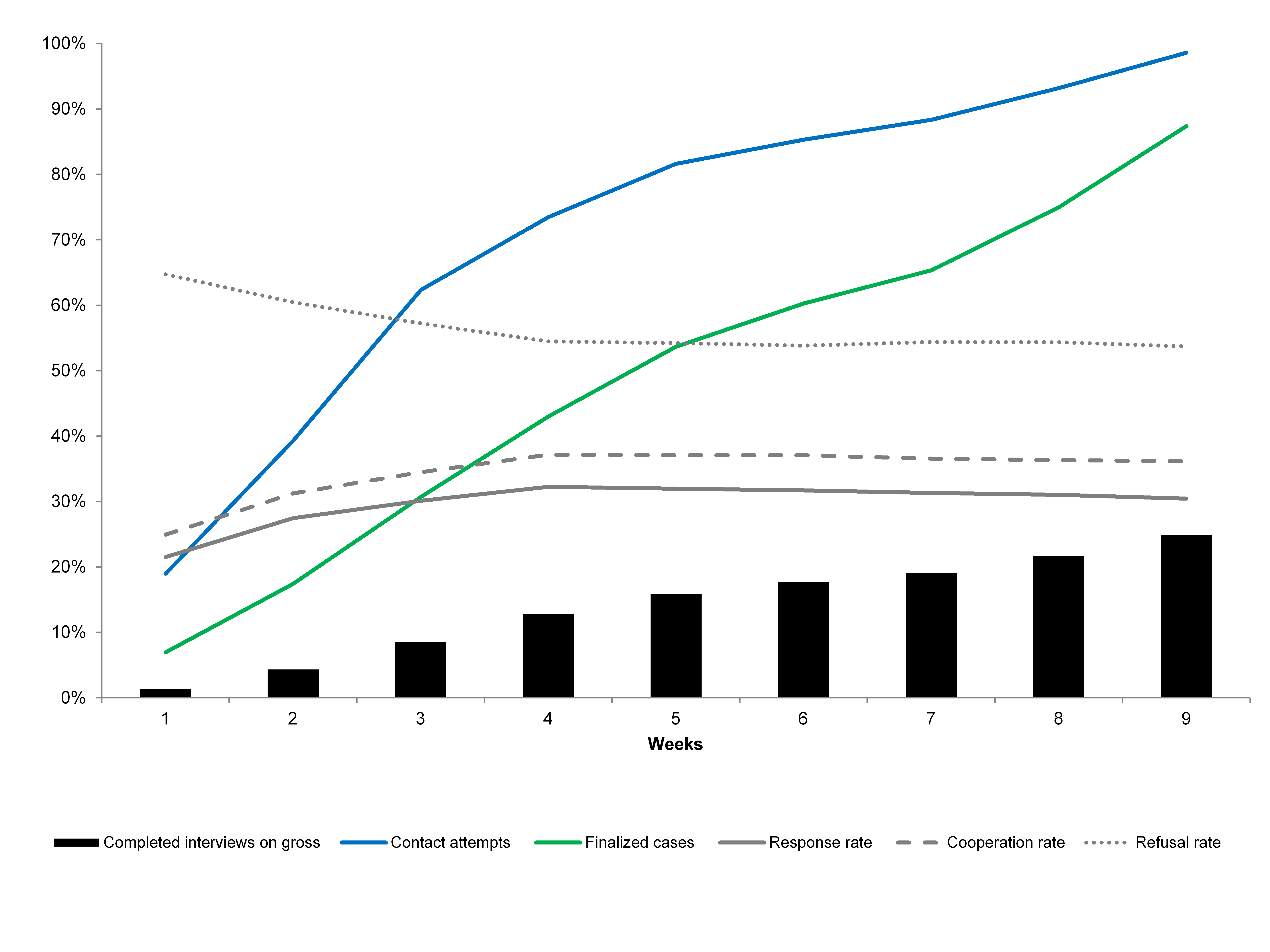
Figure 1 shows these rates and parameters for the GLES post-election cross-sectional survey. The black bars show the proportion of conducted interviews on the gross. Clearly, the proportion of interviews conducted continuously increased until week nine. The blue line shows the proportion of target persons (cases) with a contact attempt. Ideally, this line would quickly increase, approaching 100 percent, which would indicate that all addresses are processed at an early stage. However, fieldwork of GLES started rather slow: By week five, 82 percent of the target persons had been contacted in person at least once. The green line shows the proportion of finalized cases on the gross sample. Ideally, this line should be 100 percent at the end of the field period. This would mean that all addresses are finalized and that there are no more addresses with the status “work in progress”. In the case of the post-election cross-section of the GLES, this line only reaches 75 percent in week eight and 87 percent in week nine, which is sub-optimal. However, the relatively low rate can be attributed to the necessarily short and restrictive data collection period.

These parameters give an overall indication of progress during the fieldwork period. Yet, this data cannot differentiate between regions where things are going well and where they run poorly. Here, the weekly status reports can be evaluated at the federal state level to calculate identical rates at that level[1], as shown in Figure 2.

Figure 2: Indicators of the Current Fieldwork Monitoring Differentiated by Federal States

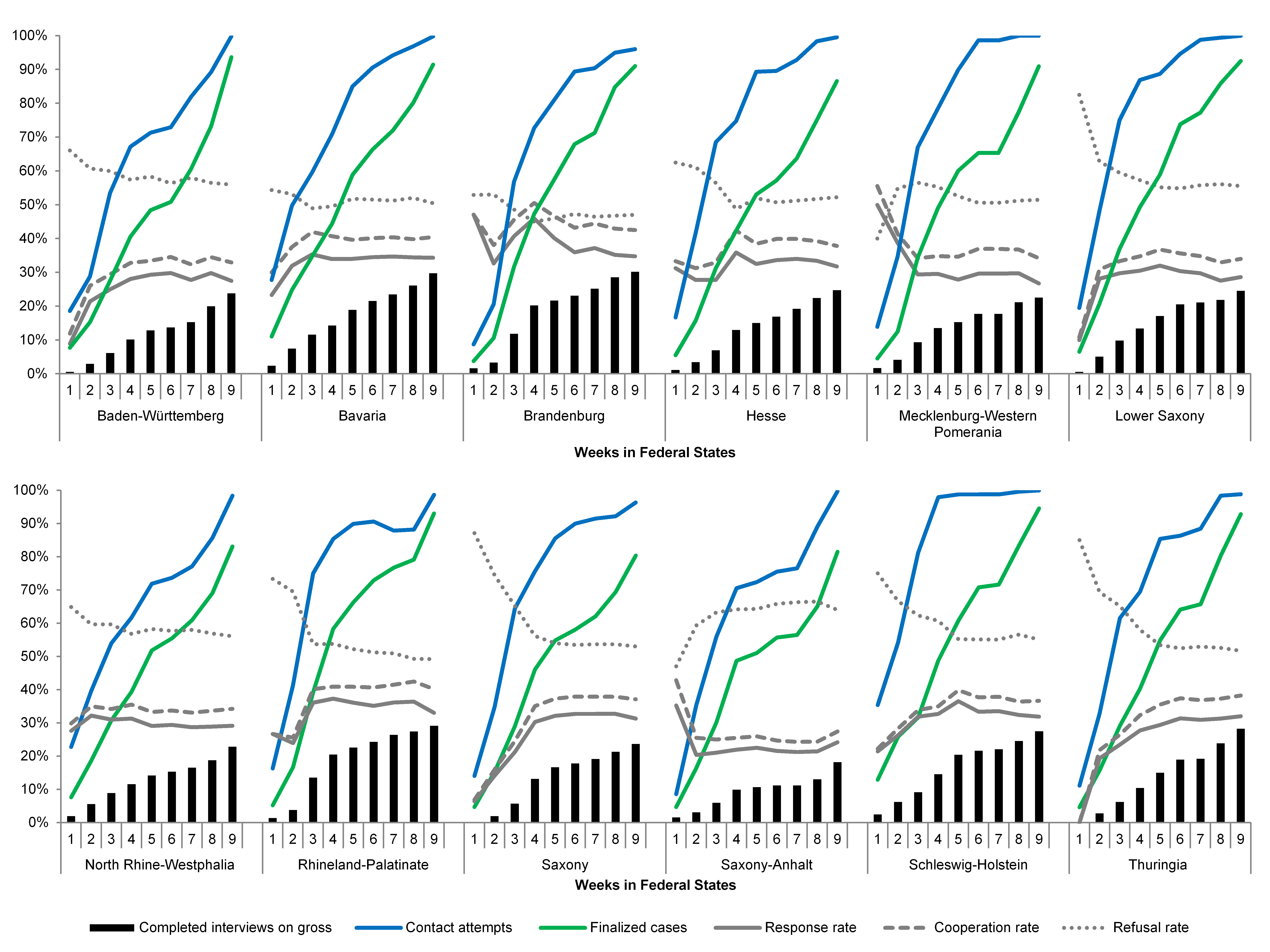
Considering the proportion of completed interviews on the gross sample, Saxony-Anhalt (18 percent) performed noticeably worse than the other states. Bavaria, Brandenburg, Rhineland-Palatinate, Schleswig-Holstein, and Thuringia finished with much better results (28-30 percent). A closer look at the blue lines in Saxony-Anhalt and in Brandenburg and Thuringia shows that the field start was quite slow in these states. The green line furthermore shows the proportion of finalized cases on the gross. Only a slowly rising line can be observed in North Rhine-Westphalia, Saxony, and Saxony-Anhalt, which means that many addresses remained unprocessed until the end of the field period in week nine, even though the interviewers’ assignment would have been to finalize all cases at the latest until the end of the field period.

In summary, the analyses at the federal state level can indicate problems in fieldwork. We know there are problems in certain states; however, we do not know whether and to what extent these problems end at administrative borders. Nevertheless, comparable calculations and graphic visualizations can be performed at the sample point or interviewer level. Given the high number of sample points and interviewers, however, the charts and tables often become cluttered and lose clarity. In addition, identifying individual interviewer IDs alone is often insufficient for understanding and solving a regional problem. Therefore, considering the geographical context is often recommended, especially in the case of reallocating interviewers. The following section presents a tool to address this problem.

5.  Tool for Geospatial Fieldwork Monitoring

5.1. Development, Objectives, and Introduction of the Tool

To address the problem described above, we propose regional visualizations. The idea is to map the addresses of important fieldwork activities using data from fieldwork monitoring. Fundamentally, the tool calculates key performance indicators based on the previously introduced weekly status report and by geographically displaying the indicators. This makes it possible to identify geographical processing problems at an early stage. A quick visual identification makes it possible to immediately recognize the underlying problems and to find a suitable solution.

It is important to emphasize three qualities of the tool that were prioritized during the development process: (1) Simplicity in use, (2) flexibility in applications, and (3) transferability to other surveys. First, the visualization tool is kept simple and can be used by anyone with experience in Stata and fieldwork monitoring. We provide the Stata file as a template to give other researchers a blueprint for their own geographic visualizations. Second, the tool is highly flexible. Every visualisation can be customized to the specific needs of the study, e.g. field characteristics, interview completion rates, or the level of fieldwork visualization (replication_code). Finally, the tool can be easily adapted to various requirements. To calculate the current field development based on the gross sample – as illustrated in the following – it is assumed that all addresses of the gross are available before the field start. However, the basic idea can also be transferred to any geographical unit (postal code, geocode data, etc.).

In most cases of face-to-face fieldwork monitoring, the results will be visualized at the community or sample point level to easily identify high-performing and, more importantly, underperforming areas. Geographical analyses at the interviewer level are also conceivable and often desirable. In our example, we present – for data protection purposes – a spatial visualization at the constituency level of administrative districts (NUTS 3). This is not problematic as the paper focuses on the general presentation of a fieldwork visualization tool and not on analyzing the performance of GLES fieldwork. In the real fieldwork monitoring of GLES, where data protection is less problematic, GLES monitors at the sample point, community, and interviewer levels.

Several indicators and indices can be calculated on the basis of the geographical data. In this paper, we present three indicators that are particularly well suited for monitoring time- and event-related studies, but can also be used in other studies:

(1) The proportion of target persons with contact attempts on the gross sample (‘contact attempts’): This indicator shows whether an interviewer is working on the address – regardless of whether this has led to success in terms of contacts or interviews or no success.

(2) The proportion of finalized cases on the gross sample of the (regional) unit we observe (‘finalized cases’). This provides information on how many cases are currently still being worked on and thus makes it possible to assess the potential that is still possible.

(3) The proportion of interviews on interviews plus refusals (‘cooperation rate’). We display this indicator because the cooperation rate in early phases of the data collection period is a good proxy for the achievable cooperation rate at the end of fieldwork.

In order to create the charts, we use the information from the weekly status report and calculate these indicators (contact attempts, finalized cases, cooperation rate), which are then aggregated and graphically presented.

5.2. Presentation and Discussion of the Geospatial Fieldwork Monitoring of GLES

In this section, we present and discuss geographic mapping. During the field period, the field agency submits weekly status reports from which the graphs can be automatically generated (after a one-time setup). This does not completely replace the tables, but easily and quickly identifies problematic regions.

The following link shows a slider with the three calculated indicators for each week. A general overview can be found in the appendix.

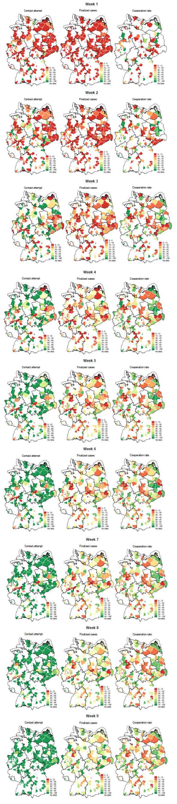
Figure 3: Geospatial Fieldwork Monitoring of GLES

 http://gesis.johannes-blumenberg.de/fieldwork/

We expect the three indicators to show differences over time. The following developments are expected for proper fieldwork, which is to be regarded as a blueprint or target value. For the coloring of the maps, we have opted for the classic traffic light system, where red indicates none or a poor processing status and green indicates a good processing status.

(1) Contact attempts: Interviewers are supposed to start their work, i.e. to visit the addresses, as quickly as possible. Accordingly, the expectation is that the “contact attempt” maps will relatively quickly change from red (attempt to contact up to 25 percent of addresses) to green (attempt to contact 90 to 100 percent of addresses).[2] This scale is variable and can be adapted according to the requirements of the study.

(2) Finalized cases: Of course, it may take some time before interviews take place because either no one is at home, the interviewer has contact with the wrong target person, or an appointment for a later time has to be made. Accordingly, the second maps should change more slowly but steadily from red (up to 5 percent of finalized cases) to green (between 40 to 100 percent of finalized cases)[3]. This scale can also be adapted according to the respective needs of a study. In this case, we chose the scale sections based on the response rate (already known).

(3) Cooperation rate: Finally, the cooperation rate shows the ratio of successful interviews to refusals plus interviews. Here, changes in the coloring are time-independent. While the first two indicators could only change in one direction (from red to green) during the data collection period, the cooperation rate can change in both directions. In a perfect world, the entire map would ultimately be green. This scale is also adaptable. In this example, red stands for a ratio of 0 to 15 percent between refusals and interviews and green stands for a ratio of 75 to 100 percent.[4]

To demonstrate the work with the tool in an exemplary way, we want to focus on nine weeks of fieldwork in a certain region. This refers to the region encompassing southern Lower Saxony and northern North Rhine-Westphalia and is highlighted by the magnifying glass on the maps.

In the first week, the regions under the magnifying glass on the “contact attempts” map are almost all red – as is also the case for most of Germany. This is unsurprising, as experience has shown that the GLES fieldwork starts slowly. Three regions near the federal state border are already colored yellow or even light green due to a comparatively high number of contact attempts. Here, the interviewers started immediately with the contact attempts. In addition, 10-15 percent of the interviews were already carried out in one of these regions, as can be seen on the “finalized cases” map. The “cooperation rate” map is not as meaningful in the first week and analysts should be cautious when interpreting it, because of the mostly small number of processed cases. However, this map can also identify areas where no interviewer activity has taken place yet. These regions remain white on the “cooperation rate” map, despite being colored on the other maps.

Maps of the following weeks show that many more addresses were processed (contact attempts, finalized cases). Indeed, some areas performed very well, and show steady changes from red to orange or yellow. The “cooperation rate” map is also informative in the first half of the fieldwork period: the interviewers are very successful in some regions (green), while they are less successful in others (red). This tendency is also evident on the first two maps. Thus, we find regions where many addresses have already been approached (“contact attempts”), but not yet been interviewed (“finalized cases”). This occurs when many addresses show contact attempts but are followed by non-contacts or refusals, which raises the following questions: Is this a problem of the region and, if so, does the interviewer need special support? Alternatively, are the interviewers ineffective and, if so, do they need additional training or should they be replaced?

Adjustments should not be made too fast. For example, an intervention after the first field week seems to be too hasty. Nevertheless, continuous visual monitoring is important, because it can function as an early warning system. However, problematic areas must be identified and appropriate steps developed and implemented in the middle of the field period, at the latest.

Examining week 4, we see that, in some areas (North Rhine-Westphalia), the proportion of “contact attempts” is lower than 50 percent (red areas). Thus, the interviewers here are still not active, which should be criticized as soon as possible.

Particularly important and problematic are those areas where many contact attempts have been made, but the cooperation rate is low or not displayed. This can also be observed in northern North Rhine-Westphalia. While in the sixth week, 90 to 100 percent of the addresses have been contacted, only 15 to 20 percent of the interviews had taken place and, accordingly, the cooperation rate is very low.

In northern North Rhine-Westphalia only 0 to 5 percent of the interviews had taken place by the end of week seven. In addition, only 70 to 80 percent of the addresses in this region were contacted. Here, an intervention is recommended. All addresses in the neighboring municipalities had already been processed, and a municipality in southern Lower Saxony has a comparatively high cooperation rate. Thus, it would be wise to bring in an interviewer with a higher success rate.

In an ideal world, all maps would be dark green by the end of the fieldwork. Nevertheless, in reality, this is often not the case, as shown by the maps of the GLES post-election cross-sectional survey. However, on the “contact attempts” map of week nine, we see that nearly every address has been processed. There are few exceptions: Regions, in which contact attempts were made with only 80 to 90 percent of the addresses and, in one district, a rate of only 60 to 70 percent. Here, the field agency should have intervened.

If homogeneous fieldwork took place, all areas should appear green on the “finalized cases” map of week 9, as the overall response rate was nearly 30 percent. There are clear differences at the end of the fieldwork period, however. In some regions the proportion of interviews is over 40 percent (dark green), while in others a significantly smaller proportion of people were interviewed. Here, orange and red areas indicate a share of less than 20 percent. Similar patterns can be detected on the third map of week 9, which shows wide variability in the cooperation rate.

The interesting question is whether the differences in response and cooperation rates between the geographical clusters are due to the inadequate case processing, individual characteristics of target persons, or structure of the area. This shows the importance of properly analyzing the cooperation rate and identifying the reasons behind it. This makes it possible to develop concrete strategies to improve fieldwork. Furthermore, this shows that the tool can be optimized by combining socio-structural and geographical information, as well as values based on past fieldwork experience, when evaluating the maps.

In summary, spatial visualization offers a new opportunity in the evaluation of fieldwork: by emphasizing the differences between districts, it is possible to reallocate interviewers from stronger to relatively poor-performing regions located nearby. If this is not possible, the researcher can request that the fieldwork agency focus more resources on those areas exhibiting poor performance. Through geographic visualization, we gain more control over the fieldwork process and can communicate the results to the decision-maker in an easy and understandable way.

6. Conclusion

The visualization method and results presented in this article are only an initial step towards showing what visualization can achieve in fieldwork monitoring. We see clear advantages in the spatial visualization of key indicators for fieldwork monitoring. This certainly does not replace the calculation of key performance indicators and figures, which record and evaluate the current status, process, and progress of fieldwork (Chapter 1), but it can provide a quick preliminary overview and then direct attention towards problematic areas.

Data visualization has clear advantages from our point of view. First, it allows for detecting the spatial aspects of fieldwork. This enables a better coordination of interviewers and, if necessary, the exchange or (re-)allocation of interviewers from high-performing regions to those that perform poorer. Second, we can display a global as well as a narrow geographic perspective to show the fieldwork in its entirety at a single glance; we also have the possibility to access problematic regions. Third, the tool is versatile. Depending on a study’s requirements, different levels (e.g. federal state, municipality, interviewer, addresses of respondents) can be visualized. The indicators, as well as the limit values (coloring), can easily be adapted to the specific requirements of a given study.

Of course, challenges still remain that must be worked out. The visualizations may lead to misjudgments if the sample points do not correspond to the interviewer, which should always be checked in advance.

Furthermore, graphic visualization always has the disadvantage that the relevance of indicators and/or areas can be over- or underestimated due to the spatial representation. Districts with a low population density could be displayed as large areas (e.g. Eastern Germany), whereby districts with a high population density – and therefore a large number of addresses to be processed – appear very small (e.g. the Ruhr region).

Also, the process of calculating indicators requires further refinement. An important next step is to add data for the sampling frame (e.g. population registers), further geographical context data (e.g. unemployment rate, GDP, community size, population density, etc.), and contact form data to explain, e.g. response rates, cooperation rates, and other indicators. With this additional information, it is easier to understand why fieldwork is performing well in some areas and not in others. In addition, information from prior waves or similar surveys can be analyzed to assess the relative success of one survey to another survey.

In general, geographical tools are particularly suitable for controlling face-to-face interviews, especially when a homogeneous field development is important. When appropriate and necessary, the geographical tool can also be transferred to any other mode if information on the time and geolocalisation of respondents or interviewers is available. Therefore, we see visualization as a support tool for monitoring fieldwork and further visualization tools should be developed in the future. This would make it possible to assess whether an interviewer works poorly or whether a region is difficult to process. The more detailed the analyses that are carried out are, the more promising the intervention measures are that are derived from them.

[1] The Saarland and the city states of Berlin, Bremen and Hamburg are not illustrated due to the small number of cases.

[2]     The scale is variable. This study uses seven steps and contains the following ranges: 0-25 percent, 25-50 percent, 50-60 percent, 60-70 percent, 70-80 percent, 80-90 percent, and 90-100 percent. White means that no data was collected.

[3]     The scale is also variable. This study uses nine steps and contains the following ranges: 0-5 percent, 5-10 percent, 10-15 percent, 15-20 percent, 20-25 percent, 25-30 percent, 30-35 percent, 35-40 percent, and 40-100 percent. White means that no data was collected.

[4]     This study uses eight steps and contains the following ranges: 0-15 percent, 15-30 percent, 30-35 percent, 35-40 percent, 40-45 percent, 45-50 percent, 50-75 percent, and 75-100 percent. White means that no data was collected.

Appendix

Figure 3: Geospatial Fieldwork Monitoring of GLES

 

 

References

1. Ackermann-Piek, D. (2018). Interviewer effects in PIAAC Germany 2012. Mannheim: Doctoral dissertation, University of Mannheim, https://madoc.bib.uni-mannheim.de/42772/1/Dissertation_Ackermann-Piek.pdf.
2. Bieber, I., & Bytzek, E. (2013). Herausforderungen und Perspektiven der empirischen Wahlforschung in Deutschland am Beispiel der German Longitudinal Election Study (GLES). Analyse & Kritik, 35(2), 341-370.
3. Beullens, K., Loosveldt, G., Vandenplas, C., & Stoop I. (2018). Response Rates in the European Social Survey: Increasing, Decreasing, or a Matter of Fieldwork Efforts? Survey Methods: Insights from the Field, https://surveyinsights.org/?p=9673.
4. Biemer, P. P. (2010). Total Survey Error – Design, Implementation, and Evaluation. Public Opinion Quarterly, 74(5), 817-848.
5. Biemer, P. P., & Caspar, R. A. (1994). Continuous Quality Improvement for Survey Operations: Some General Principles and Applications. Journal of Official Statistics 10, 307–326.
6. de Leeuw, E., Hox, J., & Luiten, A. (2018). International Nonresponse Trends across Countries and Years: An analysis of 36 years of Labour Force Survey data. Survey Insights: Methods from the Field, https://surveyinsights.org/?p=10452.
7. Eckman, S. (2014). Coverage comparison of various methods of using the postal frame for face to face surveys. Annual Conference of the American Association for Public Opinion Research, Anaheim.
8. Edwards, B., Maitland, A., & Conner, S. (2017). Measurement Error in Survey Operations Management. In: Biemer, P.P., de Leeuw, E., Eckman, S., Edwards, B., Kreuter, F., Lyberg, L.E., Tucker, N.C., West, B.T. (Eds.): Total Survey Error in Practice. New York: John Wiley & Sons, 255-277.
9. Groves, R. M., & Couper, M. P. (1998). Nonresponse in Household Interview Surveys. New York: John Wiley & Son.
10. Groves, R. M., & Heeringa, S. G. (2006). Responsive Design for Household Surveys: Tools for Actively Controlling Survey Errors and Costs. Journal of the Royal Statistical Society, 169(3), 439-457.
11. Hicks, W. D., Edwards, B., Tourangeau, K., McBride B., Harris-Kojetin, L. D., & Moos, A. J., (2010).  Using CARI Tools to Understand Measurement Error. Public Opinion Quarterly, 74(5), 985-1003.
12. Jäckle, A., Lynn, P., Sinibaldi, J., & Tipping, S. (2013). The Effect of Interviewer Experience, Attitudes, Personality and Skills on Respondent Co-operation with Face-to-Face Surveys. Survey Research Methods, 7(1), 1-15.
13. Kreuter, F., Couper, M., & Lyberg L. (2010). The use of paradata to monitor and manage survey data collection.  Section on Survey Research Methods – JSM 2010, http://www.asasrms.org/Proceedings/y2010/Files/306107_55863.pdf.
14. Loosveldt, G. (2008). Face-to-face interviews. In: de Leeuw, E. D., Hox, J. J., & Dillman, D. A. (Eds.). International handbook of survey methodology. New York, NY: Taylor & Francis Group. 201-220.
15. Maier Jæger, M. (2016). Hello Beautiful? The Effects of Interviewer Physical Attractiveness on Cooperation Rates and Survey Responses. Sociological Methods & Research, 48(1), 156-184.
16. Malter, F. (2013). Fieldwork Monitoring in the Survey of Health, Ageing and Retirement in Europe (SHARE). Survey Methods: Insights from the Field, https://surveyinsights.org/?p=1974.
17. Mitchell, S., Strobl, M., Fahrney, K., Nguyen, M., Bibb, B.; Thissen, M. R., & Stephenson, W. (2008). Using Computer Audio-Recorded Interviewing to Assess Interviewer Coding Error. Section on Survey Research Methods, AAPOR.
18. Mohadjer, L., & Edwards, B. (2018). Paradata and dashboards in PIAAC. Quality Assurance in Education, 26(2), 263-277.
19. Morganstein, D. R., & Marker, D.A. (1997). Continuous Quality Improvement in Statistical Agencies. In: Lyberg, L. E., Biemer, P. P., Collins, M., de Leeuw, E. D., Dippo, C., Schwarz, N., & Trewin, D. (Eds.). Survey Measurement and Process Quality. New York: John Wiley & Sons. 475–500.
20. Nusser, S. (2007). Using Geospatial Information Resources in Sample Surveys. Journal of Official Statistics, 23(3), 285-289.
21. Olson, K., & Wagner, J. (2013). A field experiment using GPS devices to monitor interviewer travel behavior. Paper presented at the Annual Conference of the American Association for Public Opinion Research, Boston.
22. Rogers, A., Murtaugh, M. A., Edwards, S., & Slattery, M. L. (2004). Contacting Controls: Are We Working Harder for Similar Response Rates, and Does It Make a Difference? American Journal of Epidemiology, 160(1), 85–90, http://doi.org/10.1093/aje/kwh176.
23. Roßteutscher, S., Schmitt-Beck, R., Schoen, H., Weßels, B., Wolf, C., Bieber, I., Stövsand, L.-C., Dietz, M., Scherer, P., Wagner, A., Melcher, R., & Giebler, H. (2019): Vor- und Nachwahl-Querschnitt (Kumulation) (GLES 2017). GESIS Datenarchiv, Köln. ZA6802 Datenfile Version 3.0.1.
24. Schaeffer, N. C., Dykema, J., & Maynard, D. W. (2010). Interviews and Interviewing. In: Marsden, P. V. & Wright, J. D. (Eds.). Handbook of Survey Research. Bingley, UK: Emerald Group. 438-470.
25. Schmitt-Beck, R., Rattinger, H., Roßteutscher, S., & Weßels B. (2010). Die deutsche Wahlforschung und die German Longitudinal Election Study (GLES). In: Faulbaum, F. & Wolf C. (Eds.). Gesellschaftliche Entwicklungen im Spiegel der empirischen Sozialforschung. Wiesbaden: VS Verlag für Sozialwissenschaften. 141-172.
26. Schouten, B., Shlomo, N., & Skinner, C. (2011). Indicators for Monitoring and Improving Representativeness of Response. Journal of Official Statistics, 27(2), 231-253.
27. Thissen, M. R. (2014). Computer Audio-Recorded Interviewing as a Tool for Survey Research. Social Science Computer Review, 32(1), 90-104.
28. Thissen, M. R., & Myers, S.K. (2016). Systems and processes for detecting interviewer falsification and assuring data collection quality. Statistical Journal of the IAOS, 32(3), 339-347.
29. Vercruyssen A., & Loosveldt, G. (2017). Using Google Street View to Validate Interviewers Observations and Predict Non-Response: A Test Case. Survey Research Methods, 11(3), 345-360.
30. Wagner, J., Olson K., & Edgar, M. (2017). Assessing Potential Errors in Level-of-Effort Paradata using GPD Data. Survey Research Methods, 11(3), 219-233.
31. Williams, D., & Brick, J. M. (2018). Trends in U.S. Face-to-Face Household Survey Nonresponse and Level of Effort. Journal of Survey Statistics and Methodology, 6, 186-211.